What you'll learn
- How magnetic flux and flux linkage describe “how much magnetic field passes through” a coil.
- How Faraday’s law predicts the size of an induced emf.
- How Lenz’s law gives the direction of the induced current.
- Why moving conductors and rotating coils can generate electrical energy.
Starting point: fields, area and emf
A magnetic field is a region where magnetic materials, currents, or moving charges experience a force. Its strength is described by the magnetic flux density BBB, measured in tesla, T.
An electromotive force or emf is an energy transfer per unit charge, measured in volts, V. An emf can be induced even if there is no complete circuit; a current only flows if there is a closed conducting path.
Emf is not the same as current
An induced emf can exist in an open circuit. An induced current needs both an emf and a complete conducting loop.
Magnetic flux
Imagine holding a loop of wire in a magnetic field. More field “passes through” the loop if the loop has a bigger area, the field is stronger, or the loop is turned to face the field more directly.
Magnetic flux
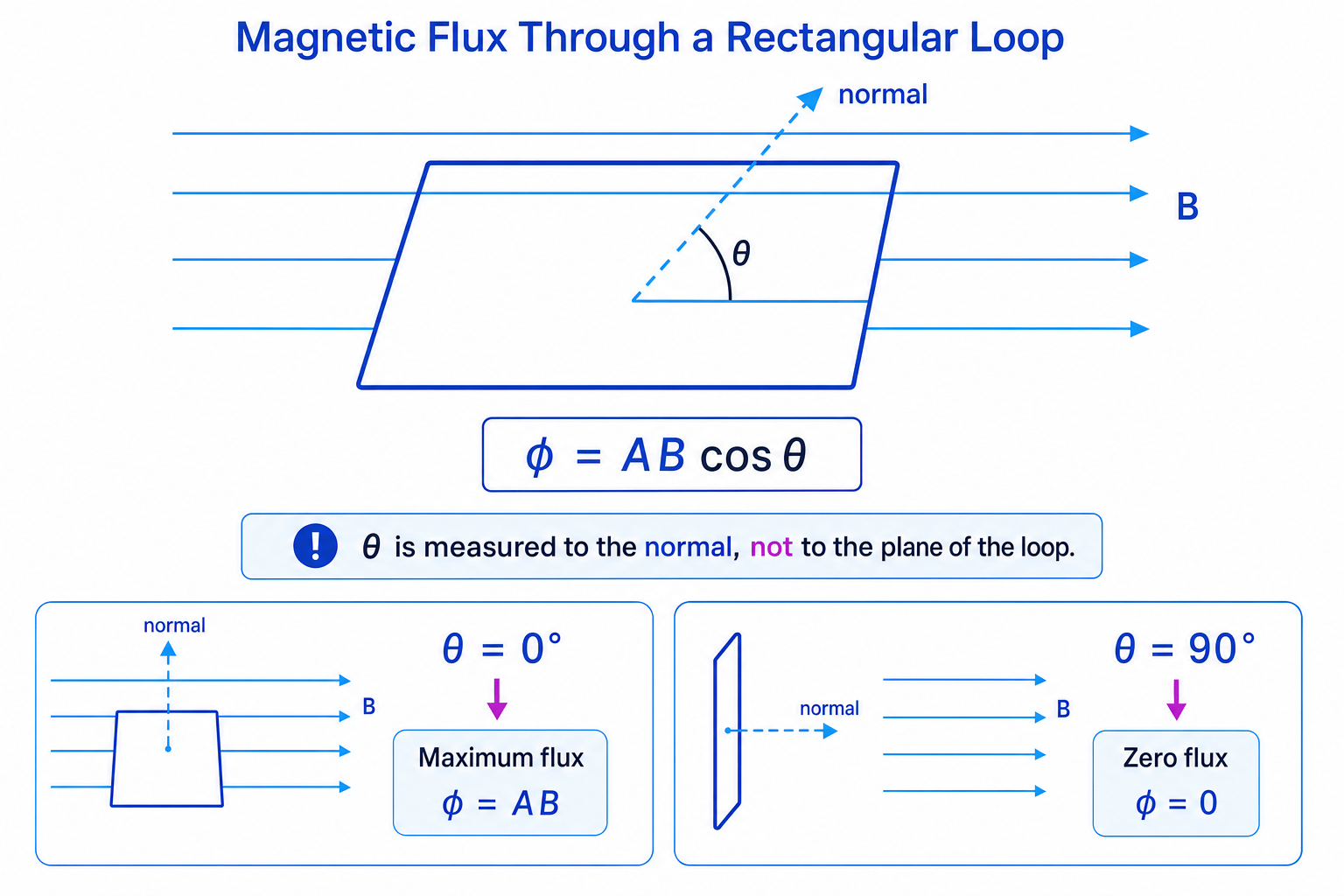
Magnetic flux ϕ\phiϕ through a flat area in a uniform magnetic field is
ϕ=ABcosθ\phi = AB\cos\thetaϕ=ABcosθwhere AAA is the area in square metres, BBB is the magnetic flux density in tesla, and θ\thetaθ is the angle between the magnetic field and the normal to the area. Magnetic flux is measured in weber, Wb, where 1 Wb=1 T m21\ \text{Wb} = 1\ \text{T m}^21 Wb=1 T m2.
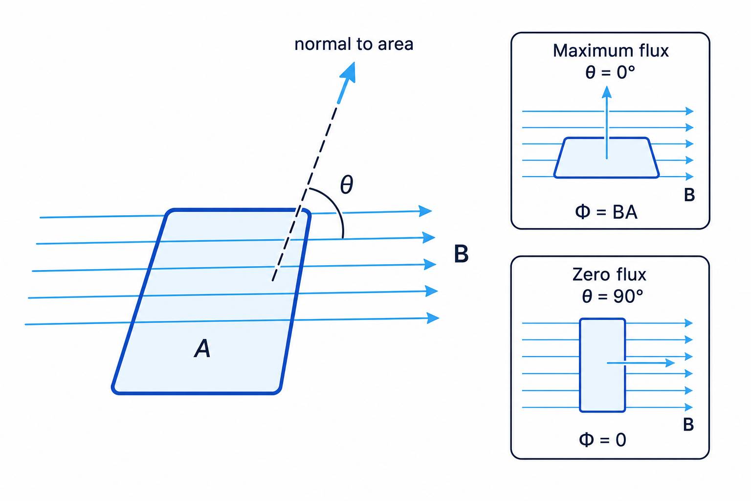
If θ=0∘\theta = 0^\circθ=0∘, the field is along the normal to the loop, so the flux is maximum: ϕ=AB\phi = ABϕ=AB. If θ=90∘\theta = 90^\circθ=90∘, the field is parallel to the plane of the loop, so no field passes through it: ϕ=0\phi = 0ϕ=0.
The angle in the flux equation
In ϕ=ABcosθ\phi = AB\cos\thetaϕ=ABcosθ, θ\thetaθ is the angle between BBB and the normal to the area, not the plane of the coil. If a question gives the angle to the plane, convert it first.
Flux linkage
A coil usually has many turns. If each turn links the same flux, the total is called the flux linkage.
Flux linkage
For a coil of NNN turns, the flux linkage is
Nϕ=NBAcosθN\phi = NBA\cos\thetaNϕ=NBAcosθIt is often quoted in weber turns, Wb turns. A “turn” is just a count, so dimensionally it is still based on weber.
Calculating flux linkage
A coil has 200 turns and area 4.0×10⁻³ m24.0 \times 10^{-3}\ \text{m}^24.0×10⁻³ m2. It is placed in a uniform magnetic field of flux density 0.25 T0.25\ \text{T}0.25 T, with the normal to the coil at 60∘60^\circ60∘ to the field.
-
Calculate the flux through one turn using the angle to the normal:
ϕ=ABcosθ=(4.0×10⁻³ m2)(0.25 T)cos60∘\phi = AB\cos\theta = \left(4.0 \times 10^{-3}\ \text{m}^2\right)\left(0.25\ \text{T}\right)\cos 60^\circϕ=ABcosθ=(4.0×10⁻³ m2)(0.25 T)cos60∘ -
Evaluate the flux:
ϕ=5.0×10⁻⁴ Wb\phi = 5.0 \times 10^{-4}\ \text{Wb}ϕ=5.0×10⁻⁴ Wb -
Multiply by the number of turns:
Nϕ=200(5.0×10⁻⁴ Wb)=0.10 Wb turnsN\phi = 200\left(5.0 \times 10^{-4}\ \text{Wb}\right) = 0.10\ \text{Wb turns}Nϕ=200(5.0×10⁻⁴ Wb)=0.10 Wb turns
Inducing an emf: Faraday’s law
An emf is induced when the flux linkage changes. You can change flux linkage by changing the magnetic flux density, the area of the loop, the angle of the loop, or by moving a coil into or out of a field.
Faraday's law
Faraday’s law says that the induced emf is equal to the negative rate of change of flux linkage:
ϵ=−Δ(Nϕ)Δt\epsilon = -\frac{\Delta(N\phi)}{\Delta t}ϵ=−ΔtΔ(Nϕ)The emf ϵ\epsilonϵ is measured in volts, V. Since 1 V=1 Wb s−11\ \text{V} = 1\ \text{Wb s}^{-1}1 V=1 Wb s−1, this equation also links weber to volt seconds.
The size of the induced emf depends on how quickly flux linkage changes. A rapid change gives a large emf; a slow change gives a small emf.
Finding average induced emf
A 250-turn coil of area 3.0×10⁻³ m23.0 \times 10^{-3}\ \text{m}^23.0×10⁻³ m2 is pulled completely out of a uniform magnetic field of flux density 0.40 T0.40\ \text{T}0.40 T. Initially the normal to the coil is parallel to the field. The coil is removed in 0.15 s.
-
Find the initial flux linkage:
Nϕi=NBAcos0∘=250(0.40 T)(3.0×10⁻³ m2)=0.30 Wb turnsN\phi_i = NBA\cos 0^\circ = 250\left(0.40\ \text{T}\right)\left(3.0 \times 10^{-3}\ \text{m}^2\right) = 0.30\ \text{Wb turns}Nϕi=NBAcos0∘=250(0.40 T)(3.0×10⁻³ m2)=0.30 Wb turns -
The final flux linkage is zero, so the change is
Δ(Nϕ)=0−0.30 Wb turns=−0.30 Wb turns\Delta(N\phi) = 0 - 0.30\ \text{Wb turns} = -0.30\ \text{Wb turns}Δ(Nϕ)=0−0.30 Wb turns=−0.30 Wb turns -
Apply Faraday’s law:
ϵ=−−0.30 Wb turns0.15 s=2.0 V\epsilon = -\frac{-0.30\ \text{Wb turns}}{0.15\ \text{s}} = 2.0\ \text{V}ϵ=−0.15 s−0.30 Wb turns=2.0 V
Lenz’s law: the direction of the induced effect
Faraday’s law gives the magnitude of the emf. Lenz’s law gives the direction.
Lenz's law
Lenz’s law says that the direction of the induced emf, and any induced current, is such that it opposes the change that produced it.
The negative sign in Faraday’s law is Lenz’s law in mathematical form. It is not “just a minus sign”; it represents energy conservation. If induced currents helped the change that produced them, you could get energy from nowhere.
Using Lenz's law for direction
A north pole of a magnet is moved towards the left-hand end of a coil connected in a complete circuit. Find the induced current direction as viewed from the magnet.
-
The approaching north pole increases the magnetic flux through the coil due to the magnet.
-
To oppose this increase, the near end of the coil must become a north pole, so it repels the approaching north pole.
-
Viewed from that end, an anticlockwise current makes the face of a coil a north pole. So the induced current is anticlockwise as viewed from the magnet.
A reliable Lenz's law routine
For direction questions, always state the change first: “the flux into the page is increasing” or “the flux to the right is decreasing”. Then choose the induced field that opposes that change.
Practical evidence and graph interpretation
A simple demonstration uses a coil connected to a sensitive voltmeter or data logger. When a magnet is stationary near the coil, there is no induced emf because the flux linkage is constant. When the magnet moves into the coil, the voltmeter deflects one way. When it moves out, it deflects the opposite way.
In practical questions, larger peak emf is produced by moving the magnet faster, using more turns, using a stronger magnet, or using a coil with a larger effective area.
If you are given a graph of flux linkage against time, the induced emf is the negative gradient:
ϵ=−Δ(Nϕ)Δt\epsilon = -\frac{\Delta(N\phi)}{\Delta t}ϵ=−ΔtΔ(Nϕ)For experimental analysis, a plot of peak emf against speed should be a straight line through the origin if the geometry is fixed, because the rate of change of flux linkage is proportional to speed.
A moving conductor in a magnetic field
A straight conducting rod moving at right angles to a uniform magnetic field has an induced emf across its ends. This is often called motional emf.
As the conductor moves, free charges inside it move with velocity vvv through the magnetic field. They experience a magnetic force, so charge separates along the rod. This creates a potential difference: an induced emf.
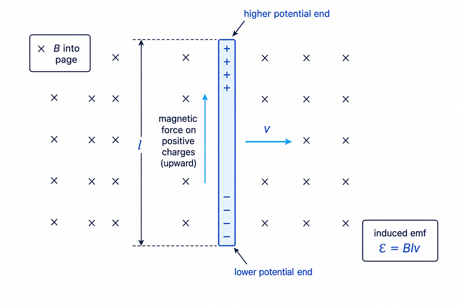
For a conductor of length lll moving at speed vvv at right angles to a uniform magnetic field:
ϵ=Blv\epsilon = Blvϵ=BlvYou can also derive this from Faraday’s law. In time Δt\Delta tΔt, the rod sweeps out area lvΔtlv\Delta tlvΔt. The flux change is BlvΔtBlv\Delta tBlvΔt, so the rate of change of flux is BlvBlvBlv.
Calculating motional emf
A vertical rod of length 0.25 m0.25\ \text{m}0.25 m moves at 3.2 m s−13.2\ \text{m}\ \text{s}^{-1}3.2 m s−1 through a uniform magnetic field of flux density 0.55 T0.55\ \text{T}0.55 T directed into the page. The rod is part of a circuit with total resistance 1.8 Ω1.8\ \Omega1.8 Ω.
-
Use the motional emf equation because the rod, velocity and field are mutually perpendicular:
ϵ=Blv=(0.55 T)(0.25 m)(3.2 m s−1)\epsilon = Blv = \left(0.55\ \text{T}\right)\left(0.25\ \text{m}\right)\left(3.2\ \text{m}\ \text{s}^{-1}\right)ϵ=Blv=(0.55 T)(0.25 m)(3.2 m s−1) -
Calculate the emf:
ϵ=0.44 V\epsilon = 0.44\ \text{V}ϵ=0.44 V -
If the circuit is complete, use V=IRV = IRV=IR:
I=0.44 V1.8 Ω=0.24 AI = \frac{0.44\ \text{V}}{1.8\ \Omega} = 0.24\ \text{A}I=1.8 Ω0.44 V=0.24 A
Only the perpendicular motion counts
The simple equation ϵ=Blv\epsilon = Blvϵ=Blv applies when the conductor moves at right angles to the magnetic field. If the motion is not perpendicular, only the component of velocity perpendicular to the field contributes.
Rotating coils and generators
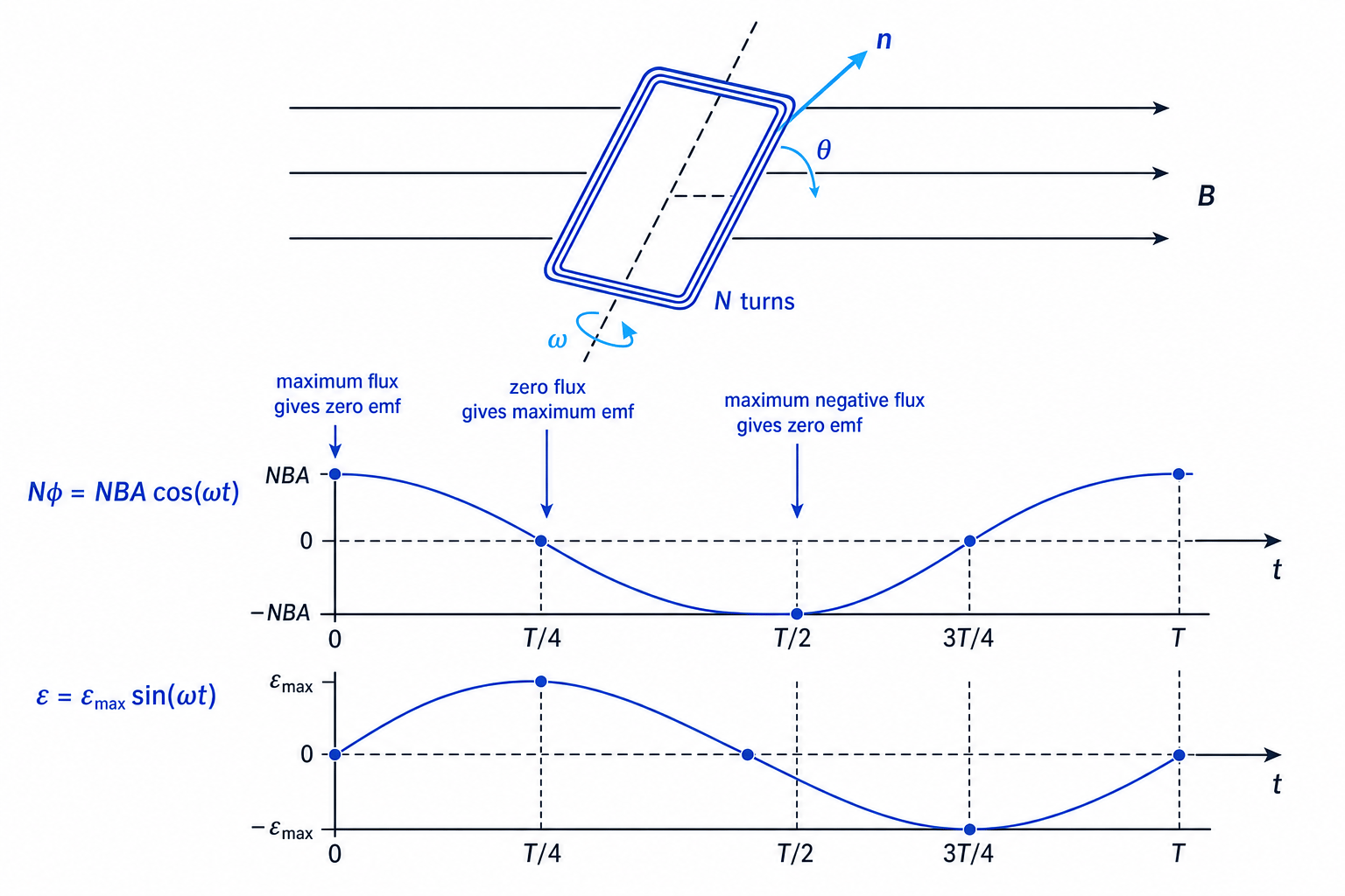
A rotating coil in a magnetic field is the basis of an a.c. generator. The coil’s flux linkage changes continuously as it rotates, so an emf is induced continuously.
If the normal to the coil makes angle θ\thetaθ with the magnetic field, then
Nϕ=NBAcosθN\phi = NBA\cos\thetaNϕ=NBAcosθFor steady rotation, θ=ωt\theta = \omega tθ=ωt, where ω\omegaω is the angular velocity in radians per second, rad s−1^{-1}−1. The flux linkage varies as a cosine curve:
Nϕ=NBAcos(ωt)N\phi = NBA\cos(\omega t)Nϕ=NBAcos(ωt)The induced emf depends on the rate of change of this flux linkage. It is zero when flux linkage is maximum, and maximum when flux linkage is changing fastest.
Position matters
When the coil is face-on to the field, flux is maximum but the induced emf is zero. When the coil is edge-on to the field, flux is zero but the induced emf is maximum.
For a coil rotating uniformly, the peak induced emf is proportional to the number of turns, flux density, area and angular velocity:
ϵmax=NBAω\epsilon_{\text{max}} = NBA\omegaϵmax=NBAωSo a larger BBB, larger AAA, more turns NNN, or faster rotation ω\omegaω gives a larger peak emf. The sign reverses every half-turn, so the output is alternating.
Estimating generator peak emf
A coil with 50 turns and area 1.2×10⁻³ m21.2 \times 10^{-3}\ \text{m}^21.2×10⁻³ m2 rotates at 25 Hz in a magnetic field of flux density 0.35 T0.35\ \text{T}0.35 T.
-
Convert frequency to angular velocity:
ω=2πf=2π(25 s−1)=157 rad s−1\omega = 2\pi f = 2\pi\left(25\ \text{s}^{-1}\right) = 157\ \text{rad s}^{-1}ω=2πf=2π(25 s−1)=157 rad s−1 -
Calculate the peak emf:
ϵmax=NBAω=50(0.35 T)(1.2×10⁻³ m2)(157 rad s−1)\epsilon_{\text{max}} = NBA\omega = 50\left(0.35\ \text{T}\right)\left(1.2 \times 10^{-3}\ \text{m}^2\right)\left(157\ \text{rad s}^{-1}\right)ϵmax=NBAω=50(0.35 T)(1.2×10⁻³ m2)(157 rad s−1) -
Quote the result sensibly:
ϵmax=3.3 V\epsilon_{\text{max}} = 3.3\ \text{V}ϵmax=3.3 V
In the exam
- For flux, check whether the given angle is to the normal or to the plane of the coil before using ϕ=ABcosθ\phi = AB\cos\thetaϕ=ABcosθ.
- For induced emf, calculate the change in flux linkage first, then divide by the time; use Lenz’s law separately for the direction.
- For rotating coils, remember: maximum flux gives zero emf, zero flux gives maximum emf, and ϵmax∝NBAω\epsilon_{\text{max}} \propto NBA\omegaϵmax∝NBAω.
Check yourself
- Why does a stationary magnet inside a coil not induce an emf?
- A coil is rotated faster in the same magnetic field. What happens to the peak emf and the frequency of the output?
- How would you decide the direction of current when a magnet is pulled away from a coil?