Springs

Welcome to your study notes on Springs! This topic forms the foundation of the Materials section of Module 3 (Forces and Motion). Here, we will transition from looking at forces acting on objects as whole systems to exploring how forces alter the internal structure and dimensions of materials themselves.

What you'll learn

The physical distinction between tensile and compressive deformation.
How Hooke's law quantitatively describes the elastic deformation of springs and wires.
How to determine the force constant from graphical and mathematical data.
The experimental techniques (PAG2) used to test and compare different materials.

1. Deforming Materials: Tensile vs. Compressive

When a single force is applied to a free body, it accelerates. However, if two equal and opposite forces are applied to a fixed body, the forces cancel out dynamically, but they still have a physical consequence: they deform the object.

Definition

Deformation

Deformation is the change in the shape or size of an object due to the application of external forces.

Depending on the direction of these opposing forces, we categorise the deformation into two types:

Tensile deformation: Occurs when two equal and opposite collinear forces pull away from each other, acting to stretch the material. This results in an extension (an increase in length).
Compressive deformation: Occurs when two equal and opposite collinear forces push towards each other, acting to squeeze the material. This results in a compression (a decrease in length).

Extension and Compression

To quantify these changes, we compare the deformed length to the original unstretched length ( $L_0$ ):

Extension ( $x$ ): If the new length of the material is $L$ , then the extension $x$ is defined as:

x = L - L_0

Compression ( $x$ ): If the material is compressed to a shorter length $L$ , the compression $x$ is:

x = L_0 - L

In both cases, we use the symbol $x$ (or sometimes $ΔL\Delta L$ ) to represent the change in length, measured in metres (m).

2. Hooke's Law and the Force Constant

In the 17th century, physicist Robert Hooke discovered that for many materials, the deformation is directly proportional to the applied force, provided the material has not been stretched too far.

Definition

Hooke's Law

Hooke's law states that the extension (or compression) of an elastic object is directly proportional to the force applied to it, provided the limit of proportionality is not exceeded.

Mathematically, we express this proportionality as $\propto x$ . By introducing a constant of proportionality, we get the fundamental equation of elastic materials:

F = k x

Where:

$F$ is the tension or applied force in newtons (N)
$x$ is the extension or compression in metres (m)
$k$ is the force constant (often called the spring constant) of the spring or wire

The Force Constant $k$

The force constant is a measure of the stiffness of the spring or material.

A higher value of $k$ means the material is stiffer; it requires a larger force to achieve the same extension.
The SI unit of $k$ is newtons per metre ( $m−1\text{N}\,\text{m}^{-1}$ ), though you will sometimes see it given in newtons per millimetre ( $mm−1\text{N}\,\text{mm}^{-1}$ ).

Common Mistake

Units of the Force Constant

Always check the units of $k$ before starting a calculation. If $k$ is in $mm−1\text{N}\,\text{mm}^{-1}$ , you must either convert your extension to millimetres or convert $k$ to $m−1\text{N}\,\text{m}^{-1}$ (where $m−11\text{ N}\,\text{mm}^{-1} = 1000\text{ N}\,\text{m}^{-1}$ ).

Let's look at how we apply this equation to a physical system.

Example

Calculating the extension of a tension spring

A vertical steel spring has an unstretched length of $cm12.5\text{ cm}$ . When a mass of $kg4.5\text{ kg}$ is suspended from its lower end, the spring stretches within its limit of proportionality. The force constant of the spring is $m−1180\text{ N}\,\text{m}^{-1}$ . Calculate the total extended length of the spring. Take $9.81\text{ m}\,\text{s}^{-2}$ .

Calculate the force applied to the spring: The force $F$ is equal to the weight of the suspended mass.

4.5\text{ kg} \times 9.81\text{ m}\,\text{s}^{-2} = 44.145\text{ N}

Calculate the extension using Hooke's law: Rearrange $F = k x$ to solve for $x$ :

\frac{F}{k} = \frac{44.145\text{ N}}{180\text{ N}\,\text{m}^{-1}} \approx 0.24525\text{ m}

Convert the units of extension to match the unstretched length: Convert $m0.24525\text{ m}$ to centimetres:

0.24525\text{ m} \times 100\text{ cm}\,\text{m}^{-1} = 24.525\text{ cm}

Calculate the total extended length: Add the extension to the original unstretched length $L_0$ :

L_0 + x = 12.5\text{ cm} + 24.525\text{ cm} = 37.025\text{ cm}

Quoting to a sensible number of significant figures (2 SF, matching the input mass of $kg4.5\text{ kg}$ ):

\approx 37\text{ cm}

3. Force-Extension Graphs

Plotting experimental data on a force-extension graph provides a visual map of a material's behaviour under load.

Key Points on a Force-Extension Graph

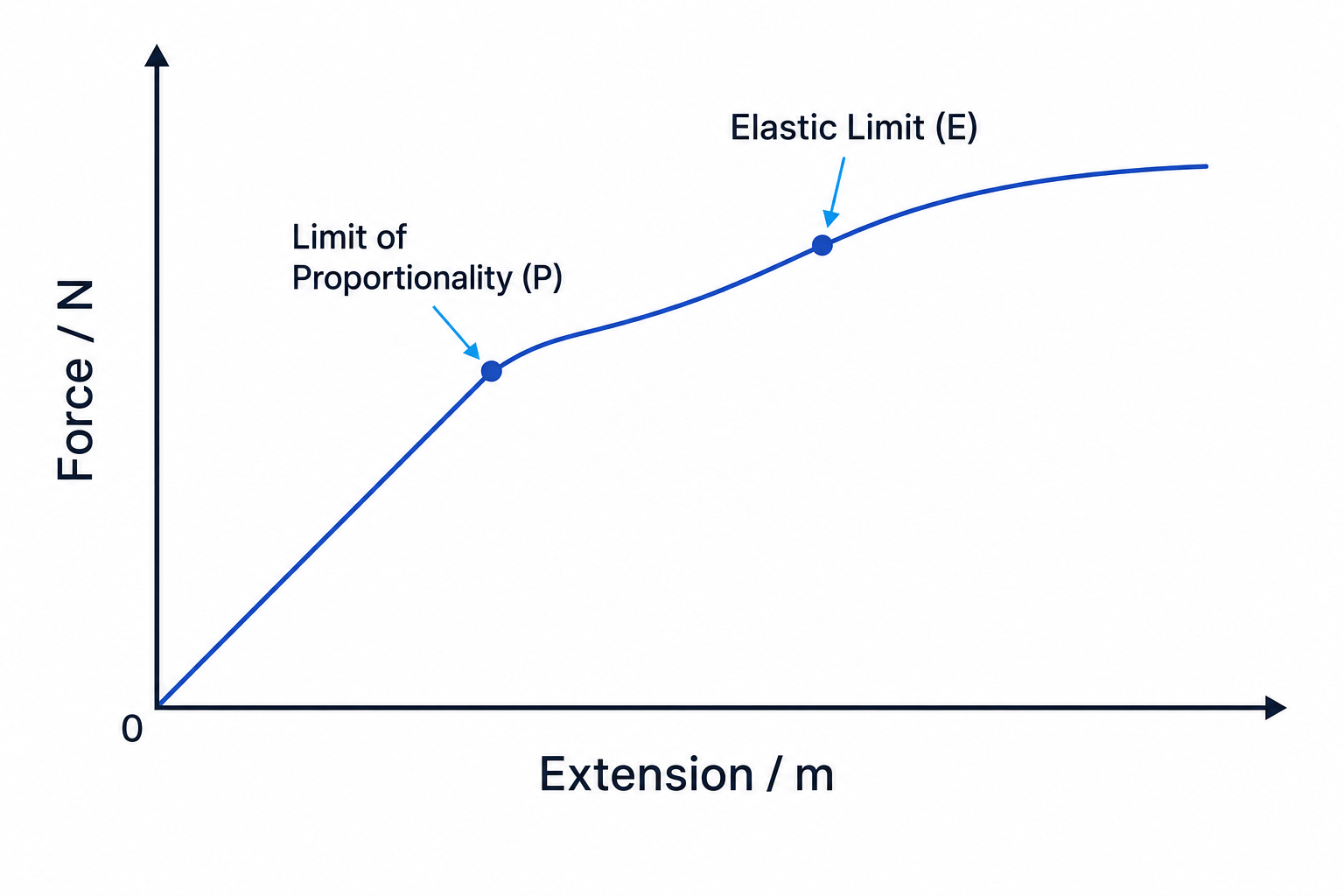
If we stretch a standard metal spring or wire, we observe several distinct regions and points on its graph:

Linear Region (Hooke's Law Region): Near the origin, the graph is a straight line passing through $(0, 0)$ . The material obeys Hooke's law here.
Limit of Proportionality (P): The point on the graph where the linear relationship stops. Beyond this point, force is no longer directly proportional to extension, and the graph begins to curve.
Elastic Limit (E): The maximum force/extension that can be applied to the material without causing permanent plastic deformation.
- If the force is removed before the elastic limit is reached, the material will return to its original length (it behaves elastically).
- If the force is removed after the elastic limit is exceeded, the material will have a permanent set; it has deformed plastically.

Force-extension graph showing limit of proportionality and elastic limit

Finding $k$ from the Graph

For the linear region of a force-extension graph (where force $F$ is on the vertical axis and extension $x$ is on the horizontal axis):

\text{Gradient} = \frac{\Delta F}{\Delta x} = k

Therefore, the gradient of the linear region equals the force constant of the spring or wire.

Common Mistake

Axes Reversal

Always check the axes of the graph in exam questions! If the graph is plotted as extension on the y-axis and force on the x-axis, the gradient is not $k$ , but $1k\frac{1}{k}$ .

4. Comparing Materials & PAG2 Investigations

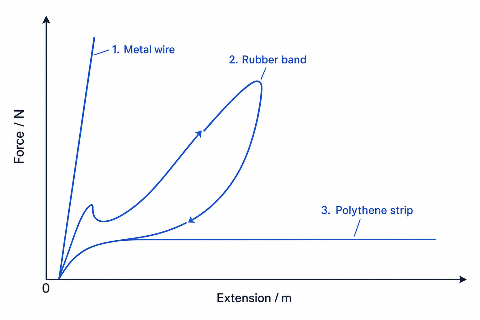
Under OCR practical requirements (PAG2), you are expected to investigate the force-extension characteristics of various materials. Three common specimens show drastically different physical behaviours:

Metal Springs or Wires: Show a clear linear region, high stiffness (steep gradient), and clear elastic and plastic regions.
Rubber Bands: Do not obey Hooke's law at all. They exhibit a curved path called a hysteresis loop. The loading curve and unloading curve do not overlap, meaning some energy is dissipated as heat. However, rubber is highly elastic and returns to its original length.
Polythene Strips: Do not obey Hooke's law. They have a very small elastic region and undergo massive plastic deformation at very low force, stretching out permanently without recovering.

Force-extension curves for different materials

Experimental Setup and Best Practice (PAG2)

To carry out a reliable investigation, you should set up your apparatus systematically to minimise uncertainties:

Support: Suspend the spring/material from a rigid clamp attached to a heavy retort stand, secured with a G-clamp to prevent it from tipping.
Measurement: Use a metre ruler aligned parallel to the spring to measure length.
Reducing Parallax Error: Fix an optical pin (or fiducial marker) horizontally to the bottom of the mass hanger. This marker should point closely to the ruler scale to ensure your eye is exactly level with the reading, avoiding parallax errors (HSW5).
Reference Point: Record the initial reading of the marker before adding any loads ( $L_0$ ).
Data Collection: Add slotted masses (e.g., $g100\text{ g}$ increments, equivalent to increments of approximately $N0.98\text{ N}$ ) and record the new position of the marker ( $L$ ). Calculate extension as $x = L - L_0$ .
Unloading: Remove masses one by one to record the unloading curve, which is essential for identifying plastic deformation or hysteresis.

Key Idea

Systematic vs Random Errors in PAG2

Systematic Error: A misaligned ruler (not perfectly vertical) will cause all length readings to be systematically overestimated. Use a set square or plumb line to ensure the ruler is vertical.
Random Error: Small fluctuations in reading the scale. Using the fiducial marker and taking multiple readings of extension on unloading and reloading can help reduce the impact of random errors.

5. Hooke's Law for Spring Combinations

While not explicitly named in every sub-bullet of the spec, the application of Hooke's law to arrangements of springs is a classic exam favourite under learning outcome (d)(ii).

Springs in Series

When springs are connected end-to-end (in series), the tension in each spring is equal to the total applied load $F$ . The total extension $x_{total}$ is the sum of the individual extensions ( $x_1 + x_2$ ).

For two springs in series with constants $k_1$ and $k_2$ :

\frac{1}{k_{total}} = \frac{1}{k_1} + \frac{1}{k_2}

Connecting springs in series makes the system less stiff (the effective $k$ decreases).

Springs in Parallel

When springs are connected side-by-side (in parallel) supporting a load together, the total load $F$ is shared between the springs ( $F_{total} = F_1 + F_2$ ), while the extension of each spring is identical ( $x_{total} = x_1 = x_2$ ).

For two springs in parallel with constants $k_1$ and $k_2$ :

k_{total} = k_1 + k_2

Connecting springs in parallel makes the system stiffer (the effective $k$ increases).

Example

Calculating the spring constant of a system

An experimental setup consists of two identical springs, each of force constant $400\text{ N}\,\text{m}^{-1}$ , connected in parallel. This parallel pair is then connected in series with a third identical spring of force constant $400\text{ N}\,\text{m}^{-1}$ . Determine the effective force constant $k_{eff}$ of the entire arrangement.

Calculate the effective force constant of the parallel pair ( $k_p$ ): Using the parallel formula:

k_p = k_1 + k_2 = 400\text{ N}\,\text{m}^{-1} + 400\text{ N}\,\text{m}^{-1} = 800\text{ N}\,\text{m}^{-1}

Combine this parallel block in series with the third spring ( $m−1k_3 = 400\text{ N}\,\text{m}^{-1}$ ): Using the series formula:

\frac{1}{k_{eff}} = \frac{1}{k_p} + \frac{1}{k_3} = \frac{1}{800\text{ N}\,\text{m}^{-1}} + \frac{1}{400\text{ N}\,\text{m}^{-1}}

Solve for $k_{eff}$ : Find a common denominator:

\frac{1}{k_{eff}} = \frac{1}{800} + \frac{2}{800} = \frac{3}{800}

Invert the expression to find $k_{eff}$ :

k_{eff} = \frac{800}{3} \approx 267\text{ N}\,\text{m}^{-1}

Exam technique

In the exam

Never forget gravity: When masses are suspended to stretch a spring, the force $F$ is the weight $W = m g$ . Make sure you use $9.81\text{ m}\,\text{s}^{-2}$ (the standard OCR value in the formula booklet) rather than $s−210\text{ m}\,\text{s}^{-2}$ .
Convert units first: Extensions are almost always recorded in millimetres ( $mm\text{mm}$ ) or centimetres ( $cm\text{cm}$ ) in lab questions, but the spring constant is standard in $m−1\text{N}\,\text{m}^{-1}$ . Convert extensions to metres ( $m1\text{ mm} = 10^{-3}\text{ m}$ ) before substituting into $F = k x$ .
Describe the graph precisely: If asked to explain the difference between the limit of proportionality and the elastic limit, make sure to state that the limit of proportionality marks the boundary of linear behaviour ( $\propto x$ ), while the elastic limit marks the boundary of reversibility (elastic vs plastic deformation).

Self review

Check yourself

A spring stretches by $cm4.0\text{ cm}$ when a $N2.0\text{ N}$ load is applied. What is its force constant in both $m−1\text{N}\,\text{m}^{-1}$ and $mm−1\text{N}\,\text{mm}^{-1}$ ?
Sketch the loading and unloading curves for a polymer material like a polythene strip, and explain why the unloading curve does not return to the origin.
Three identical springs of stiffness $k$ are connected in series. What is the effective stiffness of this system? What if they were connected in parallel?

What you'll learn

The physical distinction between tensile and compressive deformation.
How Hooke's law quantitatively describes the elastic deformation of springs and wires.
How to determine the force constant from graphical and mathematical data.
The experimental techniques (PAG2) used to test and compare different materials.