

What you'll learn
- How materials deform under tension and compression, and how to calculate the energy stored in them.
- The fundamental definitions of stress, strain, and ultimate tensile strength.
- How to measure and calculate the Young modulus of a metal using experimental techniques.
- How to distinguish between elastic and plastic deformation, and interpret stress-strain graphs for different material types.
1. Deforming Materials: Force and Extension
When a force is applied to an object, it can change its shape. In tension, forces pull the object, causing extension. In compression, forces push the object, causing it to shorten.
Force-Extension Graphs
If we apply a tensile force FFF to a material (like a wire or a spring) and measure its extension xxx, we can plot a force-extension graph.
For many materials, the initial part of this graph is a straight line through the origin. This represents Hooke's law, which states that extension is directly proportional to the applied force, provided the limit of proportionality is not exceeded:
F=kx F = kx F=kxwhere kkk is the force constant (often called the stiffness of the material or spring constant), measured in newtons per metre (N m−1\text{N}\,\text{m}^{-1}Nm−1).
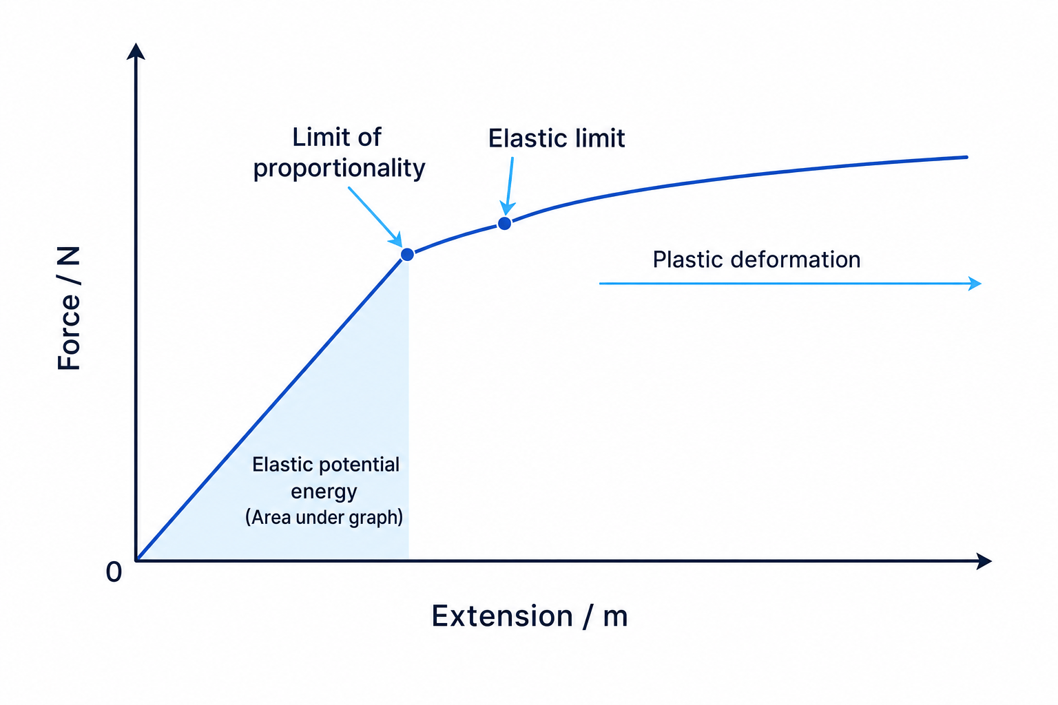
Elastic deformation
Elastic deformation is when a material returns to its original shape and length once the deforming forces (load) are removed.
Plastic deformation
Plastic deformation is when a material is permanently stretched or deformed and does not return to its original shape when the load is removed. This occurs when the load exceeds the elastic limit of the material.
Elastic Potential Energy
Work Done and Energy Stored
The work done in stretching or compressing a material is equal to the area under its force-extension (or force-compression) graph. Within the limit of proportionality, this work is stored entirely as elastic potential energy (EEE).
Mathematically, for a material obeying Hooke's law, the work done (and thus the elastic potential energy stored, EEE) is represented by the triangular area under the straight-line graph:
E=12Fx E = \frac{1}{2}Fx E=21FxSince F=kxF = kxF=kx, we can substitute this into the equation to get:
E=12kx2 E = \frac{1}{2}kx^2 E=21kx2Where:
- EEE is the elastic potential energy in joules (J\text{J}J)
- FFF is the stretching force in newtons (N\text{N}N)
- xxx is the extension in metres (m\text{m}m)
- kkk is the force constant in newtons per metre (N m−1\text{N}\,\text{m}^{-1}Nm−1)
Calculating energy stored in a spring
A steel spring has an unstretched length of 0.150 m0.150\,\text{m}0.150m and a force constant of 120 N m−1120\,\text{N}\,\text{m}^{-1}120Nm−1. Calculate the work required to stretch the spring from a length of 0.200 m0.200\,\text{m}0.200m to a length of 0.280 m0.280\,\text{m}0.280m, assuming it behaves elastically.
- Calculate the initial extension (x1x_1x1) and final extension (x2x_2x2): The extensions must be calculated from the original unstretched length (l0=0.150 ml_0 = 0.150\,\text{m}l0=0.150m):
- Calculate the initial elastic potential energy (E1E_1E1): Using the formula E=12kx2E = \frac{1}{2}kx^2E=21kx2:
- Calculate the final elastic potential energy (E2E_2E2):
- Determine the work required to stretch the spring between these two points (ΔE\Delta EΔE): The work required is the change in elastic potential energy:
Rounding to a sensible number of significant figures (2 s.f.):
ΔE≈0.86 J \Delta E \approx 0.86\,\text{J} ΔE≈0.86JIncorrect change in extension squared
When calculating the change in elastic potential energy (ΔE\Delta EΔE), a very common mistake is to square the difference in extension, i.e., writing ΔE=12k(x2−x1)2\Delta E = \frac{1}{2}k(x_2 - x_1)^2ΔE=21k(x2−x1)2. This is mathematically incorrect! You must calculate the final energy and initial energy separately and subtract them:
ΔE=12kx22−12kx12=12k(x22−x12) \Delta E = \frac{1}{2}kx_2^2 - \frac{1}{2}kx_1^2 = \frac{1}{2}k(x_2^2 - x_1^2) ΔE=21kx22−21kx12=21k(x22−x12)2. Tensile Stress and Strain
While force and extension describe a specific specimen, they depend heavily on the dimensions of the sample. To compare the mechanical properties of different materials directly, we must define scale-independent quantities: stress and strain.
Tensile stress
Tensile stress (σ\sigmaσ) is defined as the tensile force per unit cross-sectional area of a material.
σ=FA \sigma = \frac{F}{A} σ=AFWhere:
- σ\sigmaσ is stress in pascals (Pa\text{Pa}Pa or N m−2\text{N}\,\text{m}^{-2}Nm−2)
- FFF is the applied force in newtons (N\text{N}N)
- AAA is the cross-sectional area in square metres (m2\text{m}^2m2)
Tensile strain
Tensile strain (ε\varepsilonε) is defined as the extension per unit original length of a material. It is a ratio of two lengths and therefore has no units (it is dimensionless).
ε=ΔLL \varepsilon = \frac{\Delta L}{L} ε=LΔLWhere:
- ε\varepsilonε is strain
- ΔL\Delta LΔL is the extension in metres (m\text{m}m)
- LLL is the original length of the material in metres (m\text{m}m)
Ultimate Tensile Strength (UTS)
The Ultimate Tensile Strength (UTS) is the maximum tensile stress a material can withstand before it breaks or fractures. Beyond this stress level, the material will undergo "necking" (narrowing at its weakest point) and quickly snap.
3. The Young Modulus
Young Modulus
The Young modulus (EEE) is the ratio of tensile stress to tensile strain for a material within its limit of proportionality. It is a measure of the stiffness of a material.
E=stressstrain=σε E = \frac{\text{stress}}{\text{strain}} = \frac{\sigma}{\varepsilon} E=strainstress=εσBecause strain is dimensionless, the unit of the Young modulus is the same as stress: pascals (Pa\text{Pa}Pa) or newtons per square metre (N m−2\text{N}\,\text{m}^{-2}Nm−2).
We can combine the expressions for stress and strain to form a single equation for the Young modulus:
E=F/AΔL/L=FLAΔL E = \frac{F / A}{\Delta L / L} = \frac{FL}{A \Delta L} E=ΔL/LF/A=AΔLFLCalculating the extension of a loaded wire
A brass wire of original length 2.5 m2.5\,\text{m}2.5m and diameter 0.60 mm0.60\,\text{mm}0.60mm is suspended vertically. A mass of 4.5 kg4.5\,\text{kg}4.5kg is hung from the free end. The Young modulus of brass is 1.0×10¹¹ Pa1.0 \times 10^{11}\,\text{Pa}1.0×10¹¹Pa. Calculate the extension of the wire. Use g=9.81 m s−2g = 9.81\,\text{m}\,\text{s}^{-2}g=9.81ms−2.
- Calculate the tensile force (tension FFF) acting on the wire: The tension is equal to the weight of the hung mass:
- Calculate the cross-sectional area (AAA) of the wire: First, find the radius rrr from the diameter d=0.60 mm=6.0×10⁻⁴ md = 0.60\,\text{mm} = 6.0 \times 10^{-4}\,\text{m}d=0.60mm=6.0×10⁻⁴m:
Now, calculate the circular area:
A=πr2=π×(3.0×10⁻⁴ m)2=2.8274×10⁻⁷ m2 A = \pi r^2 = \pi \times (3.0 \times 10^{-4}\,\text{m})^2 = 2.8274 \times 10^{-7}\,\text{m}^2 A=πr2=π×(3.0×10⁻⁴m)2=2.8274×10⁻⁷m2- Rearrange the Young modulus equation to solve for extension (ΔL\Delta LΔL):
- Substitute the known values and solve:
The extension of the wire is 3.9 mm3.9\,\text{mm}3.9mm (expressed to 2 significant figures, matched to the input data).
4. Experimental Determination of the Young Modulus
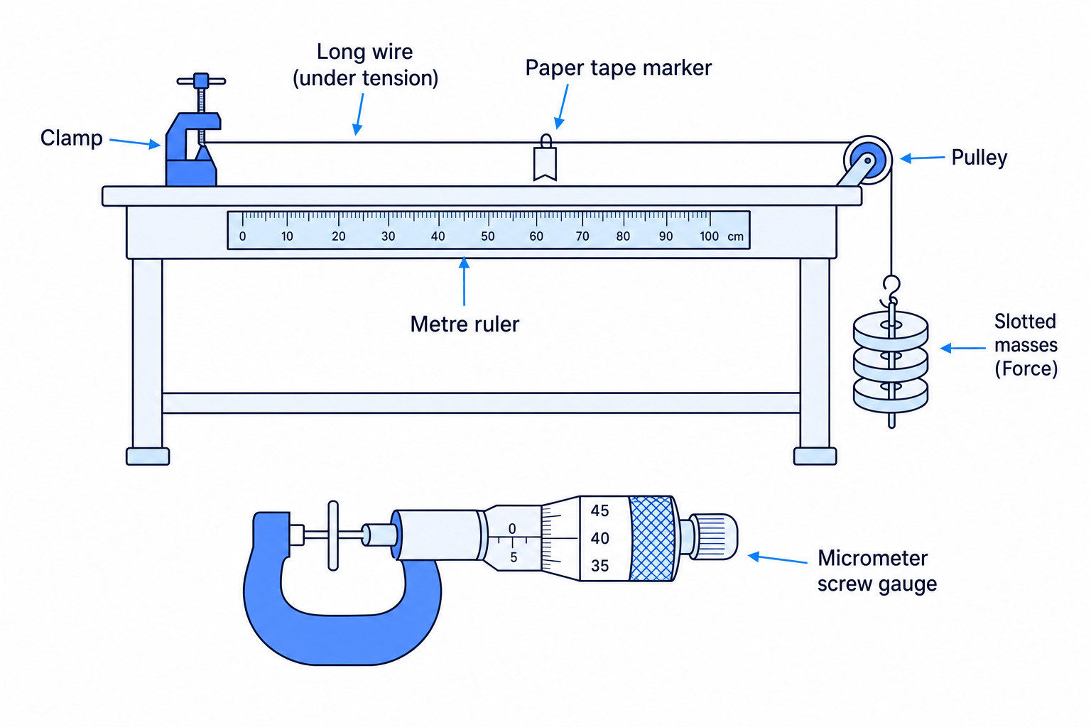
In the laboratory, you can determine the Young modulus of a metal wire using a bench-top experimental setup (aligned with Practical Activity Group 2 — PAG2).
Method and Measurements
- Measure the original length LLL: Measure the distance from the wooden clamp blocks to the paper tape marker using a metre ruler.
- Measure the wire diameter ddd: Use a micrometer screw gauge to measure the diameter of the wire at several points along its length and at different angles. Calculate the average diameter and find the area A=πd24A = \frac{\pi d^2}{4}A=4πd2.
- Add load and measure extension: Add slotted masses to the hanger, recording the force F=mgF = mgF=mg applied. For each mass, measure the new position of the paper marker on the metre ruler. Subtract the initial position to find the extension ΔL\Delta LΔL.
Minimising Uncertainties
- Long Wire: Using a very long wire (usually >2 m> 2\,\text{m}>2m) ensures that the extension ΔL\Delta LΔL is large enough to keep the percentage uncertainty in the extension reading low.
- Diameter Checks: Measuring the diameter at multiple points and angles accounts for any non-uniformity in the wire's cross-section.
- Unloading: Remove the weights in stages to ensure the marker returns to the starting position. This confirms that the wire has not undergone permanent plastic deformation.
Graphical Analysis
Since F=(EAL)ΔLF = \left( \frac{EA}{L} \right) \Delta LF=(LEA)ΔL, we can plot a graph of Force FFF (y-axis) against Extension ΔL\Delta LΔL (x-axis).
- The gradient of the linear region is equal to EAL\frac{EA}{L}LEA.
- Therefore, the Young modulus can be determined from the gradient:
Alternatively, plotting Stress σ\sigmaσ (y-axis) against Strain ε\varepsilonε (x-axis) produces a straight line through the origin where the gradient is directly equal to the Young modulus EEE.
Determining Young modulus from experimental parameters
An experiment is conducted using a copper wire of original length 2.85 m2.85\,\text{m}2.85m and diameter 0.46 mm0.46\,\text{mm}0.46mm. A plot of Force FFF against Extension ΔL\Delta LΔL yields a straight line with a gradient of 1.11×10⁴ N m−11.11 \times 10^4\,\text{N}\,\text{m}^{-1}1.11×10⁴Nm−1. Calculate the Young modulus of copper.
- Calculate the cross-sectional area of the wire: The radius is r=0.46×10⁻³ m2=2.3×10⁻⁴ mr = \frac{0.46 \times 10^{-3}\,\text{m}}{2} = 2.3 \times 10^{-4}\,\text{m}r=20.46×10⁻³m=2.3×10⁻⁴m.
- Relate the gradient of the graph to the Young modulus: Since F=(EAL)ΔLF = \left( \frac{EA}{L} \right) \Delta LF=(LEA)ΔL, the gradient of the force-extension graph is:
- Rearrange and solve for EEE:
The Young modulus of copper is 1.9×10¹¹ Pa1.9 \times 10^{11}\,\text{Pa}1.9×10¹¹Pa (or 190 GPa190\,\text{GPa}190GPa), expressed to 2 significant figures.
5. Stress-Strain Graphs for Different Materials
The shape of a stress-strain graph tells us how different classes of materials behave under load.
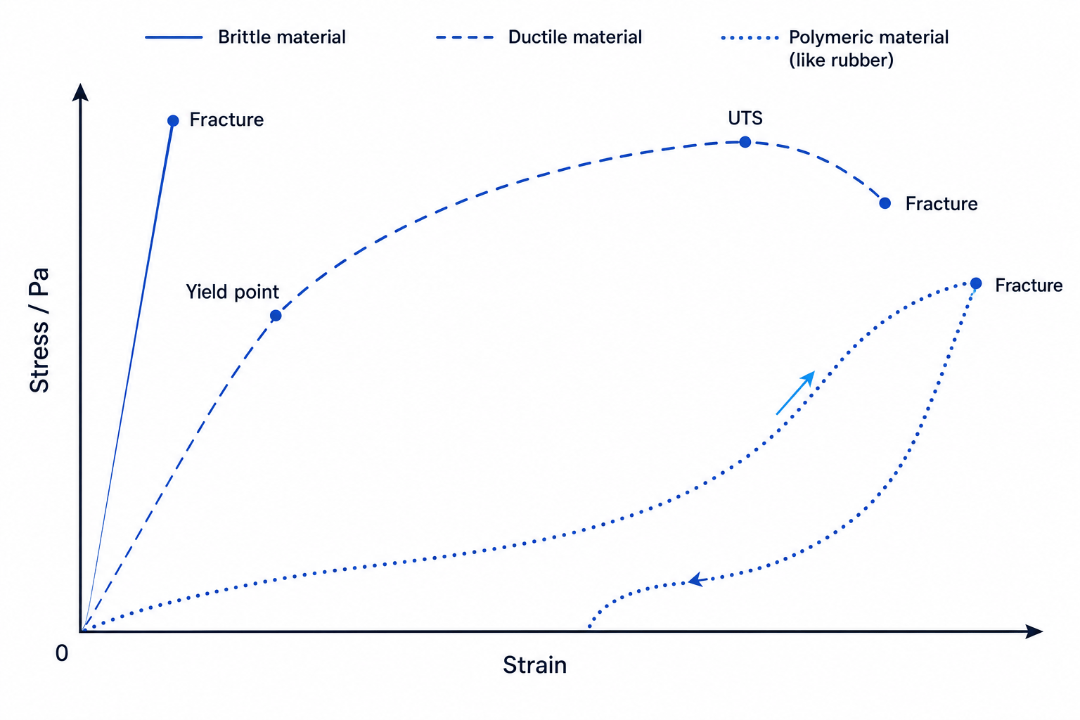
Material Classes
Ductile material
A ductile material can be drawn into wires and shows a large amount of plastic deformation before breaking (e.g., copper, mild steel).
Brittle material
A brittle material shows little or no plastic deformation. It obeys Hooke's law up to its breaking point, where it fractures suddenly (e.g., glass, cast iron).
Polymeric material
A polymeric material is made of long-chain molecules (polymers). These materials can undergo massive extensions (often elastic) and generally do not obey Hooke's law (e.g., rubber, polythene).
Rubber and Hysteresis
Rubber is a polymeric material. It can undergo massive elastic strain because its long, tangled molecular chains can easily unfold and stretch when loaded.
When rubber is loaded and then unloaded, the unloading curve lies below the loading curve. This forms a loop known as a hysteresis loop.
- The area under the loading curve represents the work done per unit volume to stretch the rubber.
- The area under the unloading curve represents the useful elastic energy returned per unit volume as it contracts.
- The area enclosed within the loop represents the mechanical energy per unit volume that is lost as thermal energy (heating up the rubber).
Calculating thermal energy dissipated in rubber hysteresis
A rubber band of unstretched length 0.12 m0.12\,\text{m}0.12m is loaded and unloaded. The area under the loading force-extension curve is 0.48 J0.48\,\text{J}0.48J. The area under the unloading curve is 0.32 J0.32\,\text{J}0.32J. Calculate: a) The work done in stretching the rubber band. b) The useful elastic energy recovered during unloading. c) The thermal energy transferred to the rubber band during this cycle.
- Identify the meaning of the area under the loading curve: The area under the loading curve represents the work done on the rubber band to stretch it:
- Identify the meaning of the area under the unloading curve: The area under the unloading curve represents the work done by the rubber band as it contracts (the useful elastic potential energy recovered):
- Calculate the thermal energy dissipated using the difference between the two areas: The energy that was put in but not recovered as mechanical work is dissipated as thermal energy (heating up the rubber band):
Units check for Stress and Young Modulus
Always check the prefix of the stress or Young modulus values in exam questions! They are usually given in megapascals (MPa=106 Pa\text{MPa} = 10^6\,\text{Pa}MPa=106Pa) or gigapascals (GPa=109 Pa\text{GPa} = 10^9\,\text{Pa}GPa=109Pa). Always convert to the base unit (Pa\text{Pa}Pa) before carrying out your calculations.
Area and radius conversions
One of the most frequent mathematical traps is converting wire diameters in millimetres (mm\text{mm}mm) to cross-sectional areas in square metres (m2\text{m}^2m2). Remember:
- Divide diameter by 2 to get radius rrr.
- Convert rrr from mm\text{mm}mm to m\text{m}m (multiply by 10−310^{-3}10−3).
- Square the radius (which squares the 10−310^{-3}10−3 conversion factor, turning it into 10−610^{-6}10−6).
- Multiply by π\piπ.
In the exam
- Always read the ruler scale direction: In Young modulus experimental questions, check if the extension measurements are cumulative or absolute positions. If positions are given, subtract the initial reading from each subsequent reading to get the true extensions.
- Distinguish force-extension vs. stress-strain: Force-extension graphs depend on the physical dimensions of the specimen. Stress-strain graphs describe the bulk material properties, meaning their gradient (Young modulus) is constant for a given material regardless of its thickness or length.
- Show all intermediate conversions: In multi-step calculation questions (like calculating extension), write down the values of cross-sectional area, force, and conversions in standard form. This secures partial marks even if you make a calculation error at the final stage.
- Learn the experimental details: Be prepared to describe how to measure the diameter of a wire (using a micrometer in multiple directions) and how to ensure the elastic limit is not exceeded (by checking if the wire returns to its original length after unloading).
Check yourself
- Can you explain the difference between the limit of proportionality and the elastic limit on a force-extension graph?
- Why is a thin, long wire preferred over a thick, short wire when setting up an experiment to determine the Young modulus of a metal?
- How is the energy dissipated per unit volume represented on a stress-strain graph for a rubber band during a loading and unloading cycle?

