Radioactivity

What you'll learn

What radioactive decay is, and why it is spontaneous and random.
How alpha, beta and gamma radiation differ in nature, range and penetration.
How to balance nuclear decay equations and use $A=λNA=\lambda N$ .
How half-life, exponential decay, spreadsheet models and radioactive dating fit together.

Radioactive decay

Some nuclei are unstable. They can become more stable by emitting radiation from the nucleus.

Definition

Radioactive decay

Radioactive decay is the spontaneous and random transformation of an unstable nucleus into a more stable nucleus, with the emission of ionising radiation.

Spontaneous means the decay is not triggered by external conditions. Heating, cooling, changing pressure, or making a chemical compound does not change when a particular nucleus decays.

Random means you cannot predict exactly when one particular nucleus will decay. However, for a large sample, the overall pattern is predictable.

Key Idea

Random, not lawless

One nucleus is unpredictable, but a large number of nuclei follows a reliable statistical decay pattern.

In experiments, random decay shows up as fluctuating count readings. That is why you take repeated readings, count for a sensible length of time, and subtract background radiation.

Alpha, beta and gamma radiation

Definition

Ionising radiation

Ionising radiation has enough energy to remove electrons from atoms, producing ions. Alpha particles, beta particles and gamma rays are all ionising.

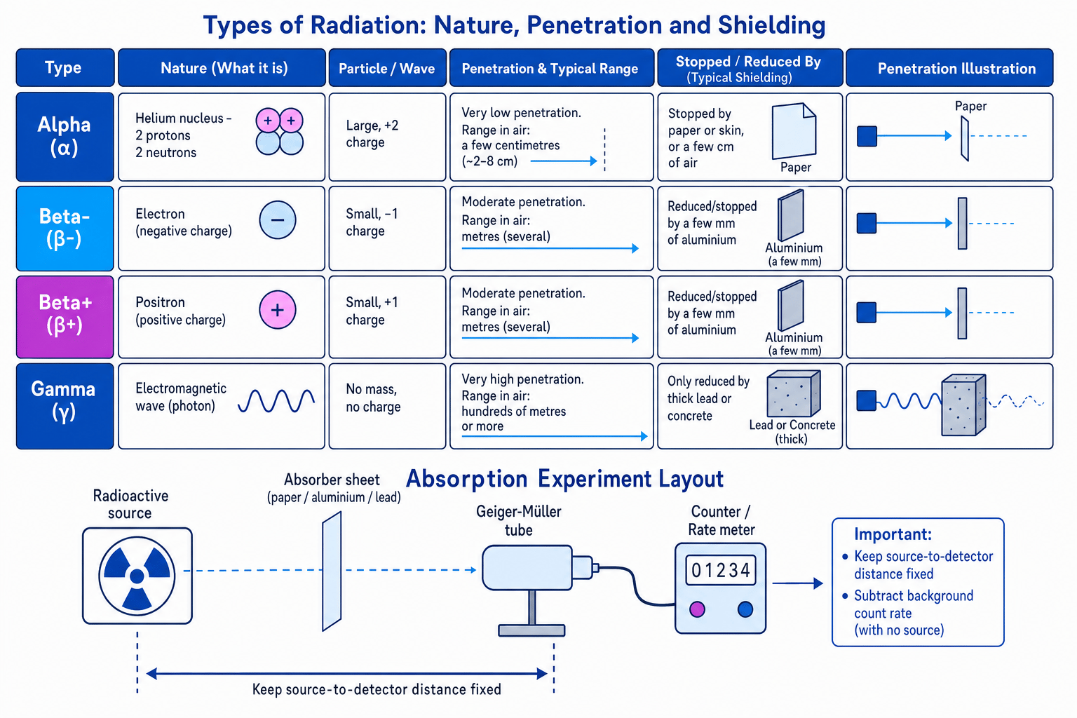
The three main nuclear radiations have different properties:

Alpha particles are helium nuclei, written as $24α{}^{4}_{2}\alpha$ or $24He{}^{4}_{2}\text{He}$ . They have charge $+ 2 e$ , are strongly ionising, and travel only a few centimetres in air. Paper or skin stops them.
Beta particles are fast electrons or positrons. A beta-minus particle is written $−10β−{}^{0}_{-1}\beta^-$ ; a beta-plus particle is written $+10β+{}^{0}_{+1}\beta^+$ . Beta radiation is moderately penetrating and is reduced or stopped by a few millimetres of aluminium.
Gamma rays are high-frequency electromagnetic waves, written $γ\gamma$ . They have no charge and no rest mass. Gamma radiation is weakly ionising but very penetrating, so thick lead or concrete is needed to reduce it significantly.

Comparison of alpha, beta and gamma radiation, showing nature, penetration, shielding, and an absorption experiment layout

Investigating absorption

To investigate absorption, you place an absorber between a radioactive source and a Geiger-Müller tube connected to a counter or rate meter.

A good procedure includes:

measuring the background count rate with no source present
keeping the source-to-detector distance fixed
using the same counting time for each reading
changing absorber material or absorber thickness
subtracting background from each measured count rate
repeating readings because radioactive decay is random

Example

Correcting an absorption measurement

A source gives 1800 counts in 60 s with no absorber. With an aluminium sheet, it gives 540 counts in 60 s. The background count is 60 counts in 60 s.

Convert each reading into a count rate:
no absorber: $1800 \div 60 = 30.0\,\mathrm{s^{-1}}$ ;
aluminium: $540 \div 60 = 9.0\,\mathrm{s^{-1}}$ ;
background: $60 \div 60 = 1.0\,\mathrm{s^{-1}}$ .
Subtract the background count rate:
no absorber: $s−130.0-1.0=29.0\,\mathrm{s^{-1}}$ ;
aluminium: $s−19.0-1.0=8.0\,\mathrm{s^{-1}}$ .
Compare the corrected rates:
transmission $\div 29.0=0.276$ , so about 28% of the original count rate remains.

Common Mistake

Forgetting background radiation

If you do not subtract background, your corrected count rate will be too high, especially when the source is weak or heavily shielded.

Nuclear decay equations

A nuclear symbol has the form $ZAX{}^{A}_{Z}X$ .

$A$ is the nucleon number: protons plus neutrons.
$Z$ is the proton number: the number of protons.
The element is determined by $Z$ .

In a nuclear equation, total nucleon number and total proton number must balance.

Alpha decay

ZAX→Z−2A−4Y+24α{}^{A}_{Z}X \to {}^{A-4}_{Z-2}Y + {}^{4}_{2}\alpha

Alpha decay reduces nucleon number by 4 and proton number by 2.

Beta-minus decay

ZAX→Z+1AY+−10β−+νˉe{}^{A}_{Z}X \to {}^{A}_{Z+1}Y + {}^{0}_{-1}\beta^- + \bar{\nu}_e

Beta-minus decay leaves nucleon number unchanged and increases the daughter proton number by 1.

Beta-plus decay

ZAX→Z−1AY++10β++νe{}^{A}_{Z}X \to {}^{A}_{Z-1}Y + {}^{0}_{+1}\beta^+ + \nu_e

Beta-plus decay leaves nucleon number unchanged and decreases the daughter proton number by 1.

Gamma emission may follow another decay. It changes the energy of the nucleus, but not $A$ or $Z$ .

Example

Balancing a beta-minus decay

Carbon-14 undergoes beta-minus decay. Balance the equation.

Start with the general beta-minus pattern:
$614C→Z14Y+−10β−+νˉe{}^{14}_{6}\text{C} \to {}^{14}_{Z}Y + {}^{0}_{-1}\beta^- + \bar{\nu}_e$ .
Balance proton number:
$6 = Z + (- 1)$ , so $Z = 7$ .
Identify the element with proton number 7: nitrogen, so
$614C→714N+−10β−+νˉe{}^{14}_{6}\text{C} \to {}^{14}_{7}\text{N}+{}^{0}_{-1}\beta^-+\bar{\nu}_e$ .

Common Mistake

Beta-minus changes the daughter nucleus upwards

In beta-minus decay, the emitted beta particle has proton number $- 1$ , so the daughter proton number increases by 1.

Activity and decay constant

Definition

Activity

The activity $A$ of a radioactive source is the number of decays per unit time. Its unit is the becquerel, where $s−11\,\mathrm{Bq}=1\,\mathrm{s^{-1}}$ .

The decay constant $λ\lambda$ is the probability per unit time that an undecayed nucleus will decay. Its unit is $s−1\mathrm{s^{-1}}$ .

For a sample containing $N$ undecayed nuclei:

A=λNA=\lambda N

A larger $λ\lambda$ means a greater probability of decay per second, so the isotope decays more quickly.

Half-life and exponential decay

Definition

Half-life

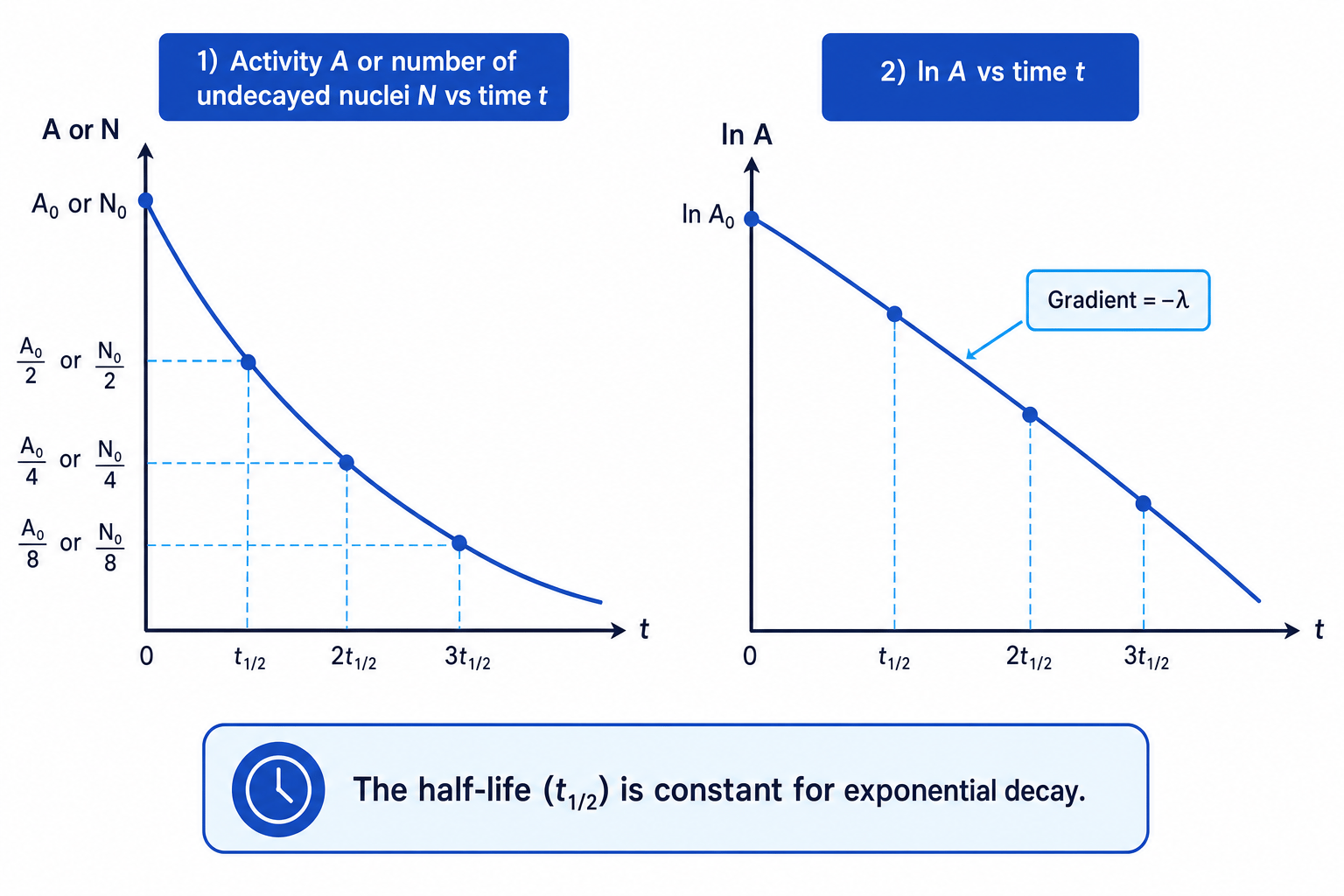
The half-life $t_{1/2}$ is the mean time taken for the activity, or the number of undecayed nuclei, to fall to half its initial value.

For radioactive decay:

λt1/2=ln⁡(2)\lambda t_{1/2}=\ln(2)

The number of undecayed nuclei and the activity both decrease exponentially:

N=N0e−λtN=N_0 e^{-\lambda t}

A=A0e−λtA=A_0 e^{-\lambda t}

Here, $N_0$ and $A_0$ are the initial number of undecayed nuclei and initial activity.

Exponential radioactive decay graph with half-life markers and a straight-line ln A against time graph

Example

Using activity, half-life and exponential decay

A sample initially contains $3.0×10163.0\times10^{16}$ undecayed nuclei. Its half-life is $s2.40\times10^{4}\,\mathrm{s}$ . Find the number of undecayed nuclei and the activity after $s7.20\times10^{4}\,\mathrm{s}$ .

Find the decay constant from the half-life:
$s−1\lambda=\ln(2)\div t_{1/2}=0.693\div(2.40\times10^{4}\,\mathrm{s})=2.89\times10^{-5}\,\mathrm{s^{-1}}$ .
Use the exponential decay equation for nuclei:
$s)=3.75×1015N=(3.0\times10^{16})e^{-(2.89\times10^{-5}\,\mathrm{s^{-1}})(7.20\times10^{4}\,\mathrm{s})}=3.75\times10^{15}$ nuclei.
Use $A=λNA=\lambda N$ :
$BqA=(2.89\times10^{-5}\,\mathrm{s^{-1}})(3.75\times10^{15})=1.08\times10^{11}\,\mathrm{Bq}$ .

Tip

Half-life sanity check

In the example, $s7.20\times10^{4}\,\mathrm{s}$ is three half-lives, so the number should be one eighth of the original. This matches $3.0×1016÷8=3.75×10153.0\times10^{16}\div8=3.75\times10^{15}$ .

Determining a half-life experimentally

For a half-life experiment, such as using a protactinium source, the count rate is proportional to activity if the geometry is kept fixed.

A typical method is:

Measure background count rate without the source.
Place the source a fixed distance from the Geiger-Müller tube.
Start timing and record counts over equal time intervals.
Subtract background from each count rate.
Plot corrected count rate against time, or plot $ln⁡A\ln A$ against time.
Find $t_{1/2}$ from repeated halvings, or use the gradient of the $ln⁡A\ln A$ graph.

If you plot $ln⁡A\ln A$ against $t$ , the gradient is $−λ-\lambda$ , so:

t1/2=ln⁡(2)λt_{1/2}=\frac{\ln(2)}{\lambda}

Common Mistake

Safety and source handling

Use the smallest suitable source, keep it in a holder, maximise distance where possible, minimise handling time, and follow the teacher’s local safety instructions.

Dice simulation of radioactive decay

A dice simulation models random decay without using radioactive material.

Each die represents one undecayed nucleus. On each throw, a chosen face, such as a six, represents decay. Dice that “decay” are removed. The number remaining is recorded after each throw.

The decay is random for each die, but the overall number remaining decreases approximately exponentially.

Example

Predicting the average dice remaining

A simulation starts with 1000 dice. A die is removed if it lands on a six.

The probability of not decaying in one throw is $5÷65\div6$ .
After four throws, the expected number remaining is
$1000(56)4=4821000\left(\frac{5}{6}\right)^4=482$ dice to three significant figures.
A real trial may not give exactly 482 because the process is random, but repeated trials would average close to this value.

Spreadsheet modelling and graphs

The finite-difference form of radioactive decay is:

ΔNΔt=−λN\frac{\Delta N}{\Delta t}=-\lambda N

The negative sign means the number of undecayed nuclei decreases.

A spreadsheet model can use columns for time, current $N$ , change $ΔN\Delta N$ , and next $N$ . For a small time step $Δt\Delta t$ :

ΔN=−λNΔt\Delta N=-\lambda N\Delta t

Nnext=N+ΔNN_{\text{next}}=N+\Delta N

Example

Updating one spreadsheet row

At one row of a model, $N = 5000$ , $s−1\lambda=0.030\,\mathrm{s^{-1}}$ , and $s\Delta t=1.0\,\mathrm{s}$ .

Calculate the change in the number of undecayed nuclei:
$s)=−150\Delta N=-(0.030\,\mathrm{s^{-1}})(5000)(1.0\,\mathrm{s})=-150$ .
Add the change to the current number:
$Nnext=5000+(−150)=4850N_{\text{next}}=5000+(-150)=4850$ .
Repeating this row-by-row produces a decreasing curve; using a smaller $Δt\Delta t$ gives a smoother approximation to exponential decay.

Graphically, a plot of $N$ or $A$ against time gives a curve. A plot of $ln⁡N\ln N$ or $ln⁡A\ln A$ against time gives a straight line with gradient $−λ-\lambda$ .

Radioactive dating

Radioactive dating uses the remaining activity of a radioactive isotope to estimate age.

In carbon dating, living material continually exchanges carbon with the environment. After death, no new carbon is taken in, so the carbon-14 activity falls as carbon-14 decays.

For a sample with current activity $A$ and original activity $A_0$ :

A=A0e−λtA=A_0e^{-\lambda t}

Rearranging gives:

t=−1λln⁡(AA0)t=-\frac{1}{\lambda}\ln\left(\frac{A}{A_0}\right)

Example

Estimating a carbon date

A sample has carbon-14 activity one quarter of the activity of living material of the same carbon mass. The carbon-14 half-life is $s1.81\times10^{11}\,\mathrm{s}$ .

Calculate the decay constant:
$s−1\lambda=\ln(2)\div(1.81\times10^{11}\,\mathrm{s})=3.83\times10^{-12}\,\mathrm{s^{-1}}$ .
Use the activity ratio $A/A_0=0.25$ :
$s−1ln⁡(0.25)t=-\frac{1}{3.83\times10^{-12}\,\mathrm{s^{-1}}}\ln(0.25)$ .
Calculate the age:
$st=3.62\times10^{11}\,\mathrm{s}$ , which is about 11 500 years.

Tip

Dating assumptions

Radioactive dating assumes the original activity is known or can be estimated, and that the sample has not gained or lost the isotope after the dating clock started.

Exam technique

In the exam

Always subtract background radiation before using count rate as activity.
In nuclear equations, balance both nucleon number $A$ and proton number $Z$ .
Keep $λ\lambda$ and $t$ in consistent units, usually $s−1\mathrm{s^{-1}}$ and seconds.
For graph questions, remember that $ln⁡A\ln A$ against $t$ has gradient $−λ-\lambda$ .

Self review

Check yourself

Why can you not predict when one nucleus will decay, even though half-life is predictable for a large sample?
How do $A$ and $Z$ change in alpha, beta-minus and beta-plus decay?
What measurements and corrections are needed before using count rate to find half-life?

What you'll learn

What radioactive decay is, and why it is spontaneous and random.
How alpha, beta and gamma radiation differ in nature, range and penetration.
How to balance nuclear decay equations and use $A=λNA=\lambda N$ .
How half-life, exponential decay, spreadsheet models and radioactive dating fit together.

Radioactive decay

Some nuclei are unstable. They can become more stable by emitting radiation from the nucleus.

Definition

Radioactive decay

Radioactive decay is the spontaneous and random transformation of an unstable nucleus into a more stable nucleus, with the emission of ionising radiation.

Spontaneous means the decay is not triggered by external conditions. Heating, cooling, changing pressure, or making a chemical compound does not change when a particular nucleus decays.

Random means you cannot predict exactly when one particular nucleus will decay. However, for a large sample, the overall pattern is predictable.

Key Idea

Random, not lawless

One nucleus is unpredictable, but a large number of nuclei follows a reliable statistical decay pattern.

In experiments, random decay shows up as fluctuating count readings. That is why you take repeated readings, count for a sensible length of time, and subtract background radiation.