

What you'll learn
- How to recognise random errors, systematic errors, and zero errors.
- The difference between precision and accuracy.
- How to calculate absolute and percentage uncertainties, then combine them in calculations.
- How to use error bars, a line of best fit, a worst acceptable line, and percentage difference.
1. Measurements are estimates
In physics, a measurement is an estimate of a physical quantity, written with a number and a unit, such as 0.248 m or 12.6 V. No measurement is perfectly exact, because instruments have limited scale divisions and experiments are affected by variation.
The true value is the value you would obtain with a perfect measurement. In real experiments, you usually do not know it exactly.
Uncertainty
An uncertainty is an estimate of the range around a measured value within which the true value is likely to lie. A result written as x±Δxx \pm \Delta xx±Δx has measured value xxx and absolute uncertainty Δx\Delta xΔx, in the same unit as xxx.
The resolution of an instrument is the smallest change it can display or that you can read from its scale. As a simple first estimate:
- an analogue scale is often read to about half the smallest division;
- a digital meter is often taken as plus/minus one in the last displayed digit, unless the instrument specification says otherwise;
- for repeated readings, the spread of values gives evidence about random uncertainty, often estimated using half the range.
The percentage uncertainty compares the absolute uncertainty with the measured value:
percentage uncertainty=Δxx×100%\text{percentage uncertainty} = \frac{\Delta x}{x} \times 100\%percentage uncertainty=xΔx×100%Calculating percentage uncertainty
A length is measured as l=(0.834±0.002) ml = (0.834 \pm 0.002)\ \text{m}l=(0.834±0.002) m.
- Identify the absolute uncertainty: Δl=0.002 m\Delta l = 0.002\ \text{m}Δl=0.002 m.
- Divide by the measured value and multiply by 100%: 0.0020.834×100%=0.2398%\frac{0.002}{0.834} \times 100\% = 0.2398\%0.8340.002×100%=0.2398%.
- Quote sensibly: the percentage uncertainty is about 0.24%.
2. Random and systematic errors
An error is the difference between a measured value and the true value. This is not quite the same as uncertainty: the error is usually unknown, while the uncertainty is your estimate of how large the error might reasonably be.
Random error
A random error causes readings to vary unpredictably about a mean value. Repeating measurements and calculating a mean reduces the effect of random errors.
Examples include reaction-time variation when using a stopwatch, small fluctuations in a meter reading, or judging a scale from slightly different angles.
Systematic error
A systematic error shifts all readings in the same direction, so the measurements are consistently too high or too low. Repeats do not remove a systematic error.
Examples include a miscalibrated voltmeter, a ruler with a worn end, or reading a scale from a fixed poor viewing angle.
A zero error is a systematic error where an instrument does not read zero when the quantity being measured is actually zero. For example, a micrometer might read 0.03 mm even when fully closed.
Zero correction
For a zero error, use:
xcorrected=xobserved−xzerox_{\text{corrected}} = x_{\text{observed}} - x_{\text{zero}}xcorrected=xobserved−xzeroSo if the zero reading is positive, subtract it from every observed reading.
Correcting a positive zero error
A micrometer reads 0.03 mm when fully closed. When measuring a wire, it reads 4.86 mm.
- The zero reading is positive, so the micrometer is reading too high by 0.03 mm.
- Apply the zero correction: xcorrected=4.86 mm−0.03 mmx_{\text{corrected}} = 4.86\ \text{mm} - 0.03\ \text{mm}xcorrected=4.86 mm−0.03 mm.
- The corrected diameter is 4.83 mm4.83\ \text{mm}4.83 mm.
Repeating does not fix everything
Taking more repeats helps with random errors, but it does not remove a systematic error. A badly zeroed instrument can give very precise repeated readings that are still inaccurate.
3. Precision and accuracy
Accuracy means closeness to the true value. A result is accurate if it is near the accepted or true value.
Precision means closeness of repeated readings to each other. A set of readings is precise if they have a small spread, even if they are all shifted away from the true value.
The target diagram is a useful mental model: the centre represents the true value, and each dot represents a repeated measurement.
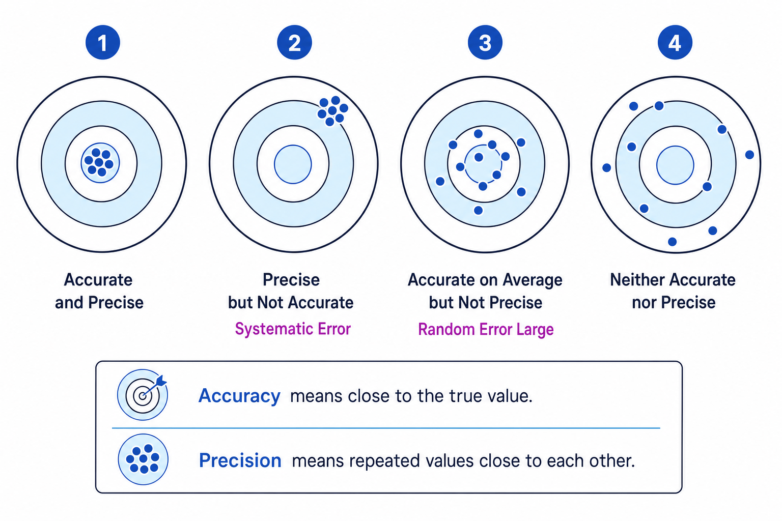
Accuracy versus precision
Random errors mainly reduce precision. Systematic errors mainly reduce accuracy.
4. Combining uncertainties
When you calculate a new quantity from measured values, the uncertainties must be combined too. At A Level, you use simple “worst-case” rules, not a full statistical treatment.
Absolute and percentage uncertainty
An absolute uncertainty has the same unit as the measurement, such as ±0.002 m\pm 0.002\ \text{m}±0.002 m. A percentage uncertainty expresses this as a percentage of the measured value.
For the simple rules below, ΔA\Delta AΔA means the absolute uncertainty in AAA.
Q=A+B or Q=A−B⇒ΔQ=ΔA+ΔBQ=AB or Q=AB⇒ΔQQ=ΔAA+ΔBBQ=An⇒ΔQQ=∣n∣ΔAA\begin{aligned} Q &= A+B\ \text{or}\ Q=A-B \quad \Rightarrow \quad \Delta Q = \Delta A + \Delta B \\ Q &= AB\ \text{or}\ Q=\frac{A}{B} \quad \Rightarrow \quad \frac{\Delta Q}{Q} = \frac{\Delta A}{A} + \frac{\Delta B}{B} \\ Q &= A^n \quad \Rightarrow \quad \frac{\Delta Q}{Q}= |n|\frac{\Delta A}{A} \end{aligned}QQQ=A+B or Q=A−B⇒ΔQ=ΔA+ΔB=AB or Q=BA⇒QΔQ=AΔA+BΔB=An⇒QΔQ=∣n∣AΔAWhich uncertainty should you add?
For addition and subtraction, add absolute uncertainties. For multiplication, division, and powers, add percentage uncertainties.
Subtracting two length readings
A marker position changes from x1=(0.112±0.001) mx_1 = (0.112 \pm 0.001)\ \text{m}x1=(0.112±0.001) m to x2=(0.284±0.001) mx_2 = (0.284 \pm 0.001)\ \text{m}x2=(0.284±0.001) m. Find the extension.
- Calculate the extension: e=x2−x1=0.284 m−0.112 m=0.172 me = x_2 - x_1 = 0.284\ \text{m} - 0.112\ \text{m} = 0.172\ \text{m}e=x2−x1=0.284 m−0.112 m=0.172 m.
- Because this is subtraction, add absolute uncertainties: Δe=0.001 m+0.001 m=0.002 m\Delta e = 0.001\ \text{m} + 0.001\ \text{m} = 0.002\ \text{m}Δe=0.001 m+0.001 m=0.002 m.
- The result is e=(0.172±0.002) me = (0.172 \pm 0.002)\ \text{m}e=(0.172±0.002) m, with percentage uncertainty 0.0020.172×100%=1.2%\frac{0.002}{0.172} \times 100\% = 1.2\%0.1720.002×100%=1.2%.
Combining multiplication, division and powers
A cylinder has mass m=(0.184±0.001) kgm = (0.184 \pm 0.001)\ \text{kg}m=(0.184±0.001) kg, radius r=(0.0120±0.0001) mr = (0.0120 \pm 0.0001)\ \text{m}r=(0.0120±0.0001) m, and length L=(0.150±0.001) mL = (0.150 \pm 0.001)\ \text{m}L=(0.150±0.001) m. Its density is ρ=mπr2L\rho = \frac{m}{\pi r^2 L}ρ=πr2Lm.
- Calculate the density: ρ=0.184π(0.0120)2(0.150)=2.71×10³ kg m−3\rho = \frac{0.184}{\pi(0.0120)^2(0.150)} = 2.71 \times 10^3\ \text{kg m}^{-3}ρ=π(0.0120)2(0.150)0.184=2.71×10³ kg m−3.
- Add percentage uncertainties, remembering that r2r^2r2 doubles the percentage uncertainty in rrr: 0.0010.184×100%+2(0.00010.0120×100%)+0.0010.150×100%=2.9%\frac{0.001}{0.184}\times100\% + 2\left(\frac{0.0001}{0.0120}\times100\%\right) + \frac{0.001}{0.150}\times100\% = 2.9\%0.1840.001×100%+2(0.01200.0001×100%)+0.1500.001×100%=2.9%.
- Convert back to an absolute uncertainty: 0.029×2.71×103 kg m−3≈0.08×10³ kg m−30.029 \times 2.71 \times 10^3\ \text{kg m}^{-3} \approx 0.08 \times 10^3\ \text{kg m}^{-3}0.029×2.71×103 kg m−3≈0.08×10³ kg m−3, so ρ=(2.71±0.08)×103 kg m−3\rho = (2.71 \pm 0.08)\times10^3\ \text{kg m}^{-3}ρ=(2.71±0.08)×103 kg m−3.
Quoting final answers
Usually quote an uncertainty to one significant figure, then quote the measured value to the same decimal place as the uncertainty. If the uncertainty begins with 1 or 2, two significant figures are often sensible.
5. Graphical treatment of uncertainties
Graphs are powerful because they show both the trend and the scatter. An error bar is a line through a plotted point showing the uncertainty in that value. At A Level, you are expected to know the basic use of error bars; you are not expected to do advanced statistics.
A line of best fit is a straight line or smooth curve that represents the overall trend. It should balance the data, not simply join the points. A worst acceptable line is the steepest or shallowest line that still reasonably fits the error bars.
This graph shows how vertical error bars, a best-fit line, and worst acceptable lines are used to estimate uncertainty in a gradient.
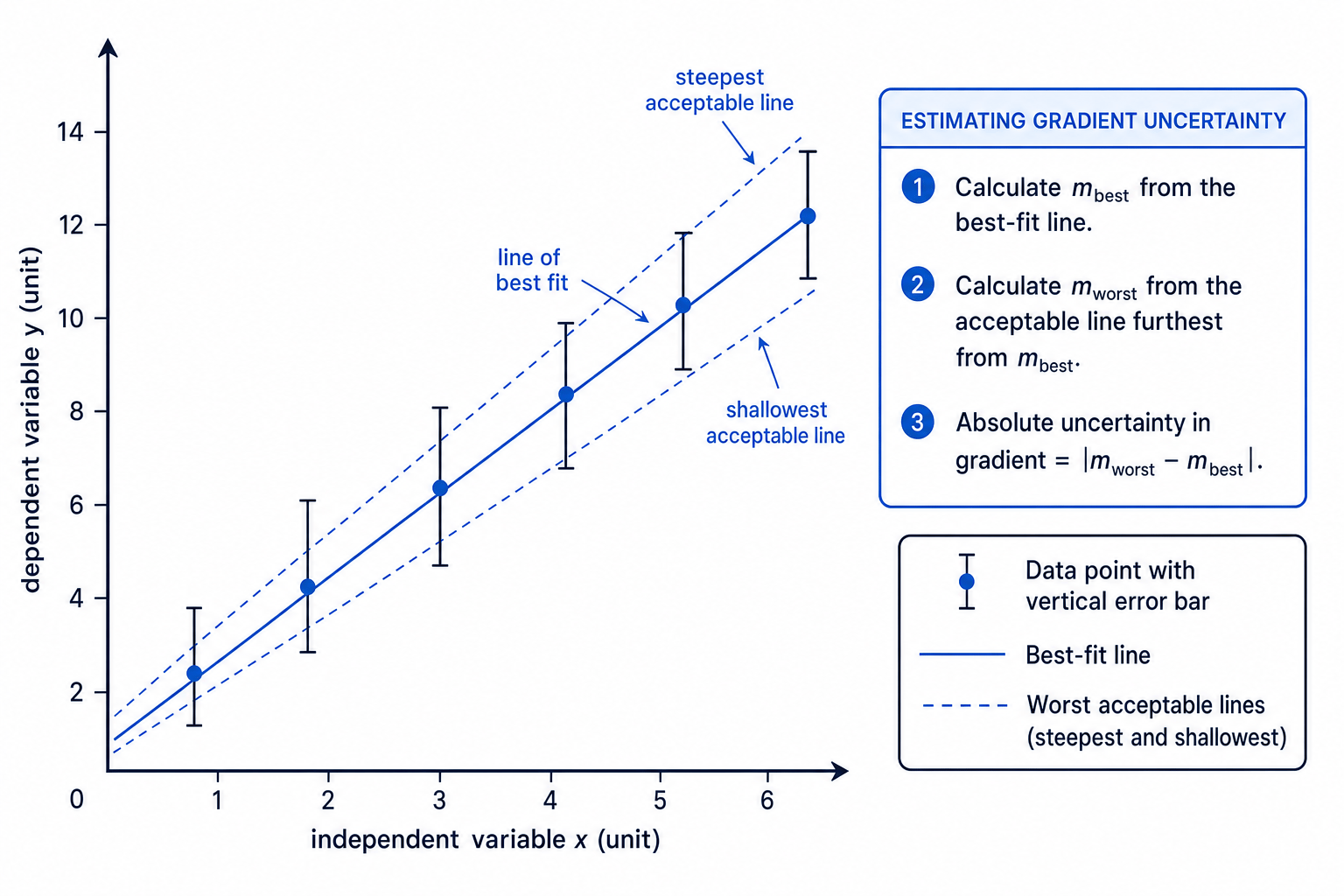
For a straight-line graph, calculate the gradient using a large triangle on the line:
gradient=ΔyΔx\text{gradient} = \frac{\Delta y}{\Delta x}gradient=ΔxΔyTo estimate uncertainty in the gradient, compare the best-fit gradient with the gradient of the worst acceptable line furthest from it:
Δm=∣mworst−mbest∣\Delta m = |m_{\text{worst}} - m_{\text{best}}|Δm=∣mworst−mbest∣Estimating uncertainty in a gradient
From a graph, the best-fit gradient is mbest=2.42 N m−1m_{\text{best}} = 2.42\ \text{N m}^{-1}mbest=2.42 N m−1. The steepest acceptable gradient is 2.58 N m−12.58\ \text{N m}^{-1}2.58 N m−1 and the shallowest acceptable gradient is 2.29 N m−12.29\ \text{N m}^{-1}2.29 N m−1.
- Compare the two possible differences: ∣2.58−2.42∣=0.16 N m−1|2.58 - 2.42| = 0.16\ \text{N m}^{-1}∣2.58−2.42∣=0.16 N m−1 and ∣2.42−2.29∣=0.13 N m−1|2.42 - 2.29| = 0.13\ \text{N m}^{-1}∣2.42−2.29∣=0.13 N m−1.
- Choose the larger difference as the absolute uncertainty: Δm=0.16 N m−1\Delta m = 0.16\ \text{N m}^{-1}Δm=0.16 N m−1.
- Calculate the percentage uncertainty: 0.162.42×100%=6.6%\frac{0.16}{2.42}\times100\% = 6.6\%2.420.16×100%=6.6%, so m=(2.42±0.16) N m−1m = (2.42 \pm 0.16)\ \text{N m}^{-1}m=(2.42±0.16) N m−1.
Forcing the line through the origin
Only force a graph through the origin if the physics requires it. Otherwise, draw the line that best represents the data and their error bars.
6. Percentage difference
A percentage difference is used to compare two values, often your experimental result with an accepted reference value.
percentage difference=∣experimental value−reference value∣reference value×100%\text{percentage difference} = \frac{|\text{experimental value} - \text{reference value}|}{\text{reference value}} \times 100\%percentage difference=reference value∣experimental value−reference value∣×100%If there is no accepted reference value and you are comparing two experimental values, follow the question wording; some questions use the mean of the two values as the denominator.
Checking agreement with an accepted value
An experiment gives gexp=(9.67±0.15) m s−2g_{\text{exp}} = (9.67 \pm 0.15)\ \text{m s}^{-2}gexp=(9.67±0.15) m s−2. The accepted value is 9.81 m s−29.81\ \text{m s}^{-2}9.81 m s−2.
- Calculate the percentage difference: ∣9.67−9.81∣9.81×100%=1.4%\frac{|9.67 - 9.81|}{9.81}\times100\% = 1.4\%9.81∣9.67−9.81∣×100%=1.4%.
- Calculate the percentage uncertainty in the experimental value: 0.159.67×100%=1.6%\frac{0.15}{9.67}\times100\% = 1.6\%9.670.15×100%=1.6%.
- Since the percentage difference is smaller than the percentage uncertainty, the result is consistent with the accepted value.
In the exam
- For error questions, state both the type of error and the remedy: repeat and average for random errors; calibrate or correct for systematic and zero errors.
- For uncertainty calculations, choose the rule before calculating: absolute uncertainties for addition/subtraction; percentage uncertainties for multiplication/division/powers.
- For graph questions, draw clear error bars, a balanced best-fit line, and a justified worst acceptable line; use a large gradient triangle and include units.
Check yourself
- A micrometer reads 0.02 mm when fully closed. What correction should you apply to a measured reading?
- For R=VIR = \frac{V}{I}R=IV, should you add absolute uncertainties or percentage uncertainties?
- How would you estimate the uncertainty in a gradient from a graph with error bars?
