

What you'll learn
- How a capacitor charges and discharges through a resistor.
- What the time constant means, and why τ=CR\tau = CRτ=CR has units of seconds.
- How to use exponential equations for charge, potential difference and current.
- How to analyse capacitor data using meters, data-loggers, lnx\ln xlnx graphs and spreadsheet models.
The essential starting point
A capacitor stores charge on two conducting plates separated by an insulator. When it is connected in a circuit, charge can move onto or off the plates, but charge does not pass through the insulating gap.
Capacitance
The capacitance CCC of a capacitor is the charge stored per unit potential difference across it:
C=QVC = \frac{Q}{V}C=VQwhere CCC is capacitance in farads (F), QQQ is charge in coulombs (C), and VVV is potential difference in volts (V).
You will also use the circuit ideas:
- V=IRV = IRV=IR for a resistor.
- Current is the rate of flow of charge, so I=ΔQΔtI = \frac{\Delta Q}{\Delta t}I=ΔtΔQ for a small time interval.
- A resistor controls how quickly charge can move onto or off the capacitor plates.
Charging and discharging through a resistor
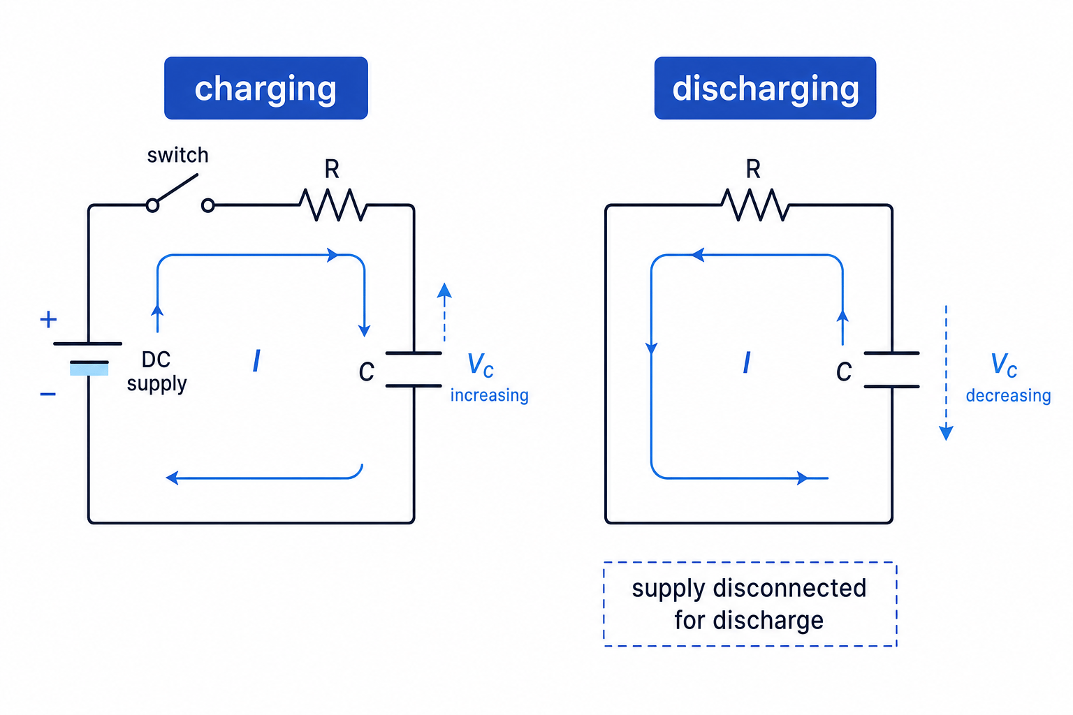
When a capacitor is charging, it is connected to a direct current supply through a resistor. At first the capacitor has little or no potential difference across it, so the current is large. As charge builds up, the capacitor potential difference increases, so the current gets smaller.
When a capacitor is discharging, the supply is removed and the charged capacitor is connected across a resistor. The capacitor now acts like a temporary source of energy, driving a current through the resistor. As it loses charge, its potential difference and current both decrease.
Shape of the change
Charging and discharging are not linear processes. The rate of change is greatest at the start, then gradually decreases, giving an exponential curve.
What changes during charging?
For a capacitor charging from zero using a supply of potential difference V0V_0V0:
- capacitor charge QQQ increases towards a maximum value Q0Q_0Q0;
- capacitor potential difference VCV_CVC increases towards V0V_0V0;
- current III starts at its maximum value and decreases towards zero.
What changes during discharging?
For a charged capacitor discharging through a resistor:
- charge QQQ decreases towards zero;
- capacitor potential difference VCV_CVC decreases towards zero;
- current III also decreases towards zero.
Thinking the current stays constant
In an RC circuit, the current is not constant. The resistor value is constant, but the capacitor potential difference changes, so the current changes with time.
Investigating capacitor charge and discharge
In the laboratory, you can investigate these curves using either meters or a data-logger.
With meters, you usually connect a voltmeter across the capacitor and record VCV_CVC at regular time intervals. Since Q=CVCQ = CV_CQ=CVC, the voltage graph has the same shape as the charge graph. You can also measure current directly with an ammeter, but capacitor currents can change quickly, so voltage measurements are often easier.
With a data-logger, a voltage sensor records VCV_CVC automatically at short time intervals. This is useful because the first part of the curve changes fastest.
Choosing component values
Pick RRR and CCC so the discharge lasts long enough to measure. A useful rule is that the main change takes about five time constants, so aim for 5CR5CR5CR to be comfortably longer than your reaction time.
For reliable results:
- use the correct capacitor polarity for electrolytic capacitors;
- discharge the capacitor fully before repeating a charging run;
- use a voltmeter or sensor with high resistance so it does not significantly discharge the capacitor;
- take more frequent readings near the start of the curve.
The time constant
Time constant
The time constant τ\tauτ of a capacitor-resistor circuit is
τ=CR\tau = CRτ=CRwhere CCC is capacitance in farads (F), RRR is resistance in ohms (Ω), and τ\tauτ is time in seconds (s).
The unit works because one ohm-farad is one second:
Ω F=VA×CV=CA=s\Omega \,\text{F} = \frac{\text{V}}{\text{A}} \times \frac{\text{C}}{\text{V}} = \frac{\text{C}}{\text{A}} = \text{s}ΩF=AV×VC=AC=sAfter one time constant:
- during discharging, QQQ, VCV_CVC or III has fallen to about 0.370.370.37 of its initial value;
- during charging, QQQ or VCV_CVC has reached about 0.630.630.63 of its final value.
After about five time constants, the capacitor is usually treated as almost fully charged or almost fully discharged.
Finding the time constant and measurement time
A 220 µF capacitor is connected in series with a 47 kΩ resistor. Estimate the time constant and the time needed for the capacitor to be nearly fully discharged.
-
Convert the component values into SI units:
C=220 μF=220×10−6 FC = 220\,\mu\text{F} = 220 \times 10^{-6}\,\text{F}C=220μF=220×10−6F R=47 kΩ=47×103 ΩR = 47\,\text{k}\Omega = 47 \times 10^3\,\OmegaR=47kΩ=47×103Ω -
Use τ=CR\tau = CRτ=CR:
τ=(220×10−6 F)(47×103 Ω)=10.34 s\tau = \left(220 \times 10^{-6}\,\text{F}\right)\left(47 \times 10^3\,\Omega\right) = 10.34\,\text{s}τ=(220×10−6F)(47×103Ω)=10.34s -
Estimate the practical discharge time as about 5τ5\tau5τ:
5τ=5×10.34 s=51.7 s5\tau = 5 \times 10.34\,\text{s} = 51.7\,\text{s}5τ=5×10.34s=51.7sSo the capacitor is nearly discharged after about 52 s.
Exponential equations for RC circuits
OCR uses equations of the form:
x=x0e−t/CRx = x_0 e^{-t/CR}x=x0e−t/CRfor discharge, and
x=x0(1−e−t/CR)x = x_0\left(1 - e^{-t/CR}\right)x=x0(1−e−t/CR)for charging.
Here xxx can represent charge QQQ, capacitor potential difference VCV_CVC, or current III, depending on the situation. The symbol x0x_0x0 means the starting value for a discharge, or the final maximum value for a charging curve.
For a discharging capacitor, the named equation is:
Q=Q0e−t/CRQ = Q_0 e^{-t/CR}Q=Q0e−t/CR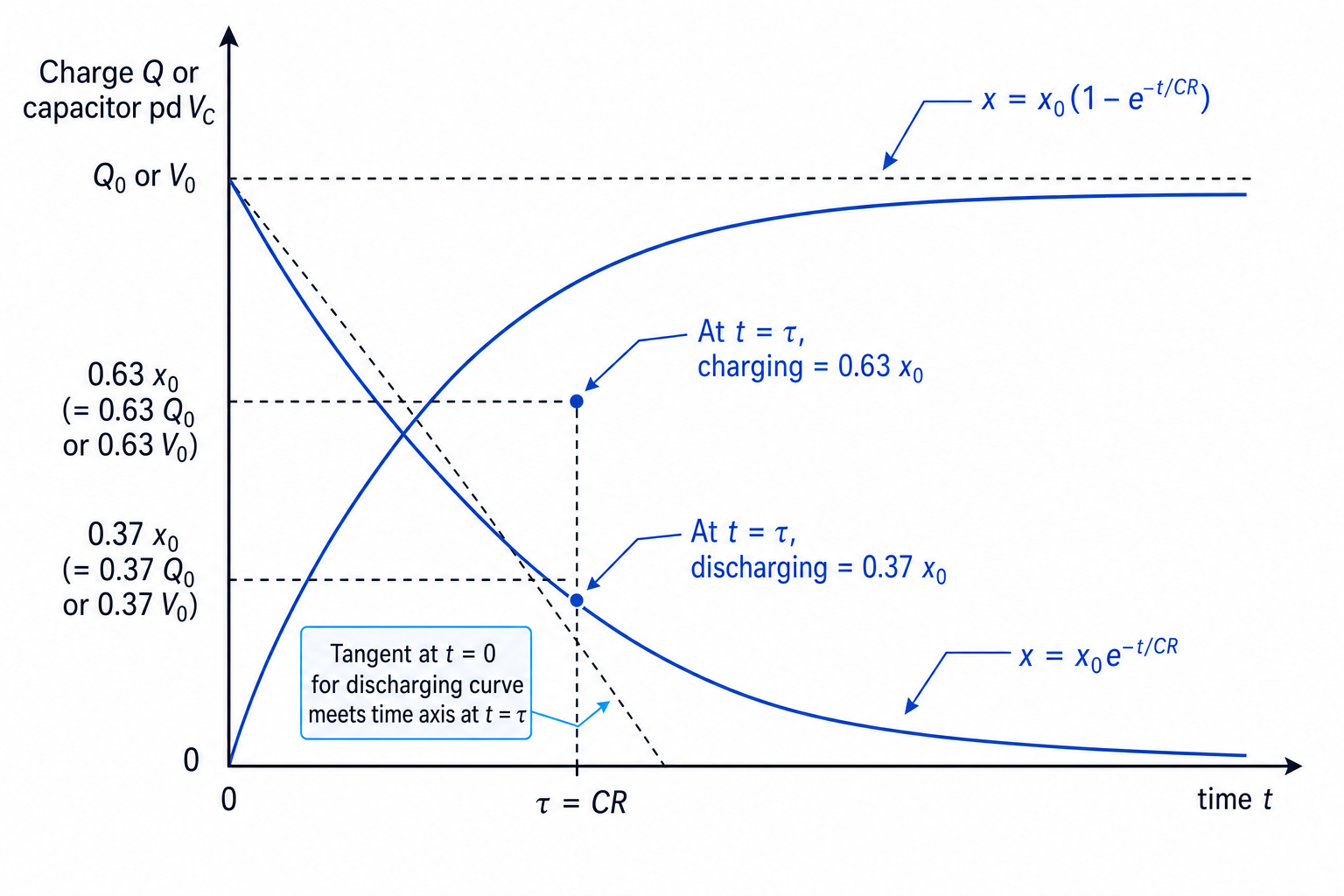
Calculating a charging voltage
A capacitor charges through a resistor from a 6.0 V supply. The circuit has R=47 kΩR = 47\,\text{k}\OmegaR=47kΩ and C=220 μFC = 220\,\mu\text{F}C=220μF. Find the capacitor potential difference after 15.0 s.
-
Calculate the time constant:
CR=(47×103 Ω)(220×10−6 F)=10.34 sCR = \left(47 \times 10^3\,\Omega\right)\left(220 \times 10^{-6}\,\text{F}\right) = 10.34\,\text{s}CR=(47×103Ω)(220×10−6F)=10.34s -
Choose the charging equation because the capacitor potential difference is increasing towards 6.0 V:
VC=V0(1−e−t/CR)V_C = V_0\left(1 - e^{-t/CR}\right)VC=V0(1−e−t/CR) -
Substitute the values:
VC=6.0 V(1−e−15.0 s/10.34 s)V_C = 6.0\,\text{V}\left(1 - e^{-15.0\,\text{s}/10.34\,\text{s}}\right)VC=6.0V(1−e−15.0s/10.34s) VC=6.0 V(1−e−1.45)=4.6 VV_C = 6.0\,\text{V}\left(1 - e^{-1.45}\right) = 4.6\,\text{V}VC=6.0V(1−e−1.45)=4.6V
Using the wrong exponential form
Use x=x0e−t/CRx = x_0e^{-t/CR}x=x0e−t/CR for a quantity that is decreasing. Use x=x0(1−e−t/CR)x = x_0(1 - e^{-t/CR})x=x0(1−e−t/CR) for a quantity that starts at zero and increases towards a maximum.
Using a lnx\ln xlnx against ttt graph
For a discharging capacitor:
x=x0e−t/CRx = x_0 e^{-t/CR}x=x0e−t/CRTaking natural logs gives:
lnx=lnx0−tCR\ln x = \ln x_0 - \frac{t}{CR}lnx=lnx0−CRtThis has the straight-line form y=mx+cy = mx + cy=mx+c:
- vertical axis: lnx\ln xlnx;
- horizontal axis: ttt;
- gradient: −1CR-\frac{1}{CR}−CR1;
- intercept: lnx0\ln x_0lnx0.
So if you plot lnVC\ln V_ClnVC against time for a discharge, the gradient lets you determine CRCRCR.
Finding CR from a logarithmic graph
A plot of lnVC\ln V_ClnVC against ttt for a discharging capacitor gives a straight line with gradient −0.125 s−1-0.125\,\text{s}^{-1}−0.125s−1. Find the time constant.
-
Match the measured gradient to the equation:
gradient=−1CR\text{gradient} = -\frac{1}{CR}gradient=−CR1 -
Rearrange for CRCRCR:
CR=−1gradientCR = -\frac{1}{\text{gradient}}CR=−gradient1 -
Substitute the gradient:
CR=−1−0.125 s−1=8.00 sCR = -\frac{1}{-0.125\,\text{s}^{-1}} = 8.00\,\text{s}CR=−−0.125s−11=8.00sThe time constant is 8.00 s.
Logs and zero readings
You cannot take ln0\ln 0ln0. For a logarithmic graph, ignore readings that have reached zero or are dominated by sensor noise.
Spreadsheet modelling of discharge
For a discharging capacitor, OCR gives:
ΔQΔt=−QCR\frac{\Delta Q}{\Delta t} = -\frac{Q}{CR}ΔtΔQ=−CRQThis says the rate of loss of charge is proportional to the charge remaining. The negative sign means QQQ is decreasing.
In a spreadsheet, use small time steps. For each row:
ΔQ=−QCRΔt\Delta Q = -\frac{Q}{CR}\Delta tΔQ=−CRQΔtthen
Qnext=Q+ΔQQ_{\text{next}} = Q + \Delta QQnext=Q+ΔQThis is a numerical model: it estimates the curve step by step. Smaller time steps usually give a better approximation to the true exponential curve.
Modelling one spreadsheet step
A capacitor has Q=24.0 mCQ = 24.0\,\text{mC}Q=24.0mC at the start of a row. The time constant is CR=10.0 sCR = 10.0\,\text{s}CR=10.0s and the spreadsheet time step is Δt=1.00 s\Delta t = 1.00\,\text{s}Δt=1.00s. Find the next charge value.
-
Convert the charge into coulombs:
Q=24.0 mC=24.0×10⁻³ CQ = 24.0\,\text{mC} = 24.0 \times 10^{-3}\,\text{C}Q=24.0mC=24.0×10⁻³C -
Calculate the change in charge during the time step:
ΔQ=−24.0×10⁻³ C10.0 s×1.00 s=−2.40×10⁻³ C\Delta Q = -\frac{24.0 \times 10^{-3}\,\text{C}}{10.0\,\text{s}} \times 1.00\,\text{s} = -2.40 \times 10^{-3}\,\text{C}ΔQ=−10.0s24.0×10−3C×1.00s=−2.40×10⁻³C -
Add the change to the old charge:
Qnext=24.0×10⁻³ C−2.40×10⁻³ C=21.6×10⁻³ CQ_{\text{next}} = 24.0 \times 10^{-3}\,\text{C} - 2.40 \times 10^{-3}\,\text{C} = 21.6 \times 10^{-3}\,\text{C}Qnext=24.0×10⁻³C−2.40×10⁻³C=21.6×10⁻³CSo the next spreadsheet value is 21.6 mC.
Time step too large
If Δt\Delta tΔt is too large compared with CRCRCR, the spreadsheet model becomes a poor approximation and can even predict unphysical negative charge values.
Constant-ratio property of exponential decay
An exponential decay has a constant-ratio property: in equal time intervals, the quantity is multiplied by the same factor.
For capacitor discharge:
xafter time Δtxbefore=e−Δt/CR\frac{x_{\text{after time } \Delta t}}{x_{\text{before}}} = e^{-\Delta t/CR}xbeforexafter time Δt=e−Δt/CRSo the graph gets flatter, but the percentage decrease over each equal time interval stays the same.
Using the constant-ratio property
A capacitor discharges with time constant 4.0 s. The initial potential difference is 8.0 V. Find the potential difference after each 2.0 s interval for the first 6.0 s.
-
Calculate the multiplying factor for each 2.0 s interval:
e−Δt/CR=e−2.0 s/4.0 s=e−0.50=0.607e^{-\Delta t/CR} = e^{-2.0\,\text{s}/4.0\,\text{s}} = e^{-0.50} = 0.607e−Δt/CR=e−2.0s/4.0s=e−0.50=0.607 -
Apply the same factor repeatedly:
V1=8.0 V×0.607=4.86 VV_1 = 8.0\,\text{V} \times 0.607 = 4.86\,\text{V}V1=8.0V×0.607=4.86V V2=4.86 V×0.607=2.95 VV_2 = 4.86\,\text{V} \times 0.607 = 2.95\,\text{V}V2=4.86V×0.607=2.95V V3=2.95 V×0.607=1.79 VV_3 = 2.95\,\text{V} \times 0.607 = 1.79\,\text{V}V3=2.95V×0.607=1.79V -
Link the results to the graph shape: the drops are 3.14 V, then 1.91 V, then 1.16 V, so the absolute decrease gets smaller even though the ratio stays constant.
In the exam
- Decide whether the quantity is charging or discharging before choosing the exponential equation.
- Calculate CRCRCR first, with RRR in ohms and CCC in farads.
- For lnx\ln xlnx graphs, remember that the gradient is negative and equals −1CR-\frac{1}{CR}−CR1.
- In practical questions, link better data to short sampling intervals, high-resistance voltmeters, repeated runs and suitable uncertainty treatment.
Check yourself
- Why is the current largest at the very start of charging or discharging?
- What fraction of the initial charge remains after one time constant during discharge?
- How would you find CRCRCR from a straight-line graph of lnVC\ln V_ClnVC against time?
