

What you'll learn
- How to process experimental observations and numerical data into valid conclusions.
- How to choose useful mathematical methods for analysing results.
- How to use significant figures sensibly in practical work.
- How to plot graphs properly and extract gradients and intercepts.
What “analysis” means in practical physics
In a practical, you do not just collect readings. You have to turn them into evidence. Analysis is the process of organising results, doing suitable calculations, plotting graphs where useful, and deciding what the results show.
Qualitative and quantitative results
Qualitative results describe observations in words, such as “the filament glowed brighter”. Quantitative results are numerical measurements with units, such as a current of 0.42 A or a length of 0.156 m.
A good analysis uses both when appropriate. A qualitative observation can help explain a pattern, but a quantitative result lets you test relationships, calculate constants and compare values.
Processing raw results
Raw and processed data
Raw data are the readings taken directly from instruments. Processed data are values calculated from raw data, such as means, gradients, percentages, reciprocals, squared values or uncertainties.
Common processing steps include:
- calculating a mean from repeat readings
- identifying anomalous results, which are readings that do not fit the pattern
- converting units into SI units
- calculating a derived quantity, such as resistance from R=VIR = \frac{V}{I}R=IV
- plotting a graph to reveal a relationship
A conclusion is only valid if it is supported by the data you actually collected. It should not claim more precision or a wider range than your experiment justifies.
Reaching a conclusion from current and potential difference data
A student measures current through a resistor at constant temperature:
- 1.0 V gives 0.20 A
- 2.0 V gives 0.39 A
- 3.0 V gives 0.61 A
- 4.0 V gives 0.80 A
Decide whether the resistor behaves ohmically over this range.
-
Use the relationship R=VIR = \frac{V}{I}R=IV to calculate resistance for each pair of readings:
R1=1.0 V0.20 A=5.0 ΩR2=2.0 V0.39 A=5.1 ΩR3=3.0 V0.61 A=4.9 ΩR4=4.0 V0.80 A=5.0 Ω\begin{aligned} R_1 &= \frac{1.0\ \text{V}}{0.20\ \text{A}} = 5.0\ \Omega \\ R_2 &= \frac{2.0\ \text{V}}{0.39\ \text{A}} = 5.1\ \Omega \\ R_3 &= \frac{3.0\ \text{V}}{0.61\ \text{A}} = 4.9\ \Omega \\ R_4 &= \frac{4.0\ \text{V}}{0.80\ \text{A}} = 5.0\ \Omega \end{aligned}R1R2R3R4=0.20 A1.0 V=5.0 Ω=0.39 A2.0 V=5.1 Ω=0.61 A3.0 V=4.9 Ω=0.80 A4.0 V=5.0 Ω -
Compare the calculated values. They are all close to 5.0 Ω, so the resistance is approximately constant.
-
State a conclusion limited to the evidence: the current is directly proportional to potential difference, so the component behaves ohmically between 1.0 V and 4.0 V, assuming its temperature remained constant.
Overstating the conclusion
Do not write “the resistor is always ohmic”. Your results only support behaviour over the measured range and under the conditions of the experiment.
Choosing the right mathematical skills
Physics analysis often means choosing the calculation that reveals the relationship. You are expected to be comfortable with skills such as rearranging equations, using ratios, calculating means, converting units, using standard form, finding gradients, and interpreting proportionality.
Let the physics equation guide the analysis
If an equation can be written in the straight-line form y=mx+cy = mx + cy=mx+c, then a graph can often turn experimental data into a value for a physical constant.
Linearising data
Linearising
Linearising means changing what you plot so that data following a curved relationship become a straight-line graph. This often involves plotting squared, square-rooted or reciprocal quantities.
For example, if a relationship is of the form m=ρVm = \rho Vm=ρV, where mmm is mass, VVV is volume and ρ\rhoρ is density, then plotting mass on the vertical axis against volume on the horizontal axis gives a straight line. The gradient is the density.
Using a gradient to find density
A graph of mass against volume for a metal has a best-fit line passing through these two points:
- volume = 2.00×10⁻⁵ m32.00 \times 10^{-5}\ \text{m}^32.00×10⁻⁵ m3, mass = 0.156 kg
- volume = 8.00×10⁻⁵ m38.00 \times 10^{-5}\ \text{m}^38.00×10⁻⁵ m3, mass = 0.624 kg
Find the density of the metal.
-
Use the straight-line equation m=ρVm = \rho Vm=ρV. Since mass is on the vertical axis and volume is on the horizontal axis, the gradient is ρ\rhoρ.
-
Calculate the gradient using two well-separated points on the best-fit line:
ρ=ΔmΔV=0.624 kg−0.156 kg8.00×10−5 m3−2.00×10⁻⁵ m3\rho = \frac{\Delta m}{\Delta V} = \frac{0.624\ \text{kg} - 0.156\ \text{kg}}{8.00 \times 10^{-5}\ \text{m}^3 - 2.00 \times 10^{-5}\ \text{m}^3}ρ=ΔVΔm=8.00×10⁻⁵ m3−2.00×10⁻⁵ m30.624 kg−0.156 kg -
Evaluate the expression with units:
ρ=0.468 kg6.00×10−5 m3=7.80×10³ kg m−3\rho = \frac{0.468\ \text{kg}}{6.00 \times 10^{-5}\ \text{m}^3} = 7.80 \times 10^3\ \text{kg m}^{-3}ρ=6.00×10⁻⁵ m30.468 kg=7.80×10³ kg m−3
Significant figures
Significant figures
Significant figures are the meaningful digits in a measured or calculated value. They show the precision justified by the data.
For example, 0.00420 m has three significant figures: 4, 2 and the final 0. The leading zeros only locate the decimal point.
In practical physics, appropriate significant figures depend on the measuring instrument and the calculation:
- Raw readings should usually be recorded to the resolution of the instrument.
- For multiplication and division, a calculated answer should usually have no more significant figures than the least precise input.
- For addition and subtraction, think about decimal places and absolute resolution.
- If quoting an uncertainty, the value and uncertainty should normally be rounded to the same decimal place.
Rounding a calculated resistance
A voltmeter reads 2.0 V and an ammeter reads 0.39 A. Calculate the resistance with an appropriate number of significant figures.
-
Substitute into R=VIR = \frac{V}{I}R=IV:
R=2.0 V0.39 AR = \frac{2.0\ \text{V}}{0.39\ \text{A}}R=0.39 A2.0 V -
Calculate the unrounded value:
R=5.128205... ΩR = 5.128205...\ \OmegaR=5.128205... Ω -
Both input readings are given to two significant figures, so quote the resistance to two significant figures:
R=5.1 ΩR = 5.1\ \OmegaR=5.1 Ω
False precision
Writing every calculator digit, such as 5.128205 Ω, suggests a precision that the experiment did not have. Rounding is part of the physics, not just presentation.
Plotting suitable graphs
Graphs are one of the most powerful analysis tools in A-Level Physics. They help you spot trends, test proportionality and calculate constants from gradients or intercepts.
Independent and dependent variables
The independent variable is the quantity you deliberately change. The dependent variable is the quantity you measure in response.
Usually, the independent variable goes on the horizontal axis and the dependent variable goes on the vertical axis. If you are trying to find a constant from a known equation, you may choose transformed axes instead.
Labelling axes
Each axis label must include:
- the quantity name
- the symbol, where useful
- the unit
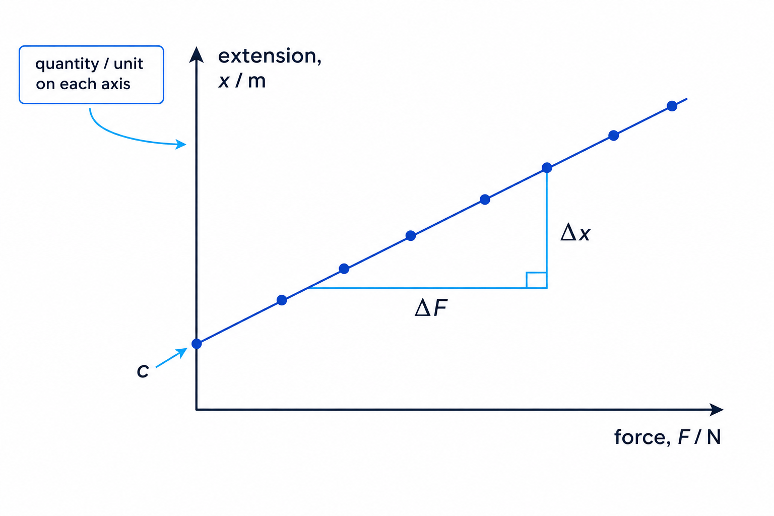
Good labels include “force, FFF / N” and “extension, xxx / m”.
Choosing scales
A suitable scale should:
- include all the data points
- use most of the graph paper
- have simple divisions, such as 1, 2 or 5 multiplied by a power of ten
- avoid awkward scales that make points difficult to plot accurately
This is what a well-annotated experimental graph looks like: data points, a best-fit line, a gradient triangle and an intercept.
Best-fit, not dot-to-dot
For experimental data, draw a smooth best-fit line or curve that follows the overall trend. Do not join points one by one unless the question specifically asks you to.
Gradients and intercepts
Gradient
The gradient of a graph is the change in the vertical-axis quantity divided by the change in the horizontal-axis quantity.
For a straight-line graph,
gradient=ΔyΔx\text{gradient} = \frac{\Delta y}{\Delta x}gradient=ΔxΔyUse a large gradient triangle drawn on the best-fit line. The points used for the gradient do not have to be original data points.
Intercept
The intercept is where the graph crosses an axis. The vertical-axis intercept is the value of yyy when x=0x = 0x=0.
The intercept can have physical meaning. For example, it may represent a zero error, an initial value or a constant term in an equation.
Finding spring constant from an extension-force graph
A student plots extension xxx against force FFF for a spring. The best-fit line passes through these two points:
- F=2.0 NF = 2.0\ \text{N}F=2.0 N, x=0.013 mx = 0.013\ \text{m}x=0.013 m
- F=8.0 NF = 8.0\ \text{N}F=8.0 N, x=0.049 mx = 0.049\ \text{m}x=0.049 m
The vertical intercept is approximately 0.001 m. Find the spring constant.
-
Start with Hooke’s law, F=kxF = kxF=kx. Since the graph is extension against force, rearrange to match the plotted axes:
x=1kF+cx = \frac{1}{k}F + cx=k1F+cSo the gradient of the graph is 1k\frac{1}{k}k1.
-
Calculate the gradient of the best-fit line:
gradient=0.049 m−0.013 m8.0 N−2.0 N=0.036 m6.0 N=0.0060 m N−1\text{gradient} = \frac{0.049\ \text{m} - 0.013\ \text{m}}{8.0\ \text{N} - 2.0\ \text{N}} = \frac{0.036\ \text{m}}{6.0\ \text{N}} = 0.0060\ \text{m N}^{-1}gradient=8.0 N−2.0 N0.049 m−0.013 m=6.0 N0.036 m=0.0060 m N−1 -
Use k=1gradientk = \frac{1}{\text{gradient}}k=gradient1:
k=10.0060 m N−1=1.7×10² N m−1k = \frac{1}{0.0060\ \text{m N}^{-1}} = 1.7 \times 10^2\ \text{N m}^{-1}k=0.0060 m N−11=1.7×10² N m−1 -
Interpret the intercept. The value 0.001 m suggests a small zero offset or initial extension, rather than a perfectly unloaded spring starting exactly at zero extension.
Gradient units missing
A gradient has units: vertical-axis unit divided by horizontal-axis unit. Missing gradient units can lose marks, especially when the gradient represents a physical constant.
In the exam
- Before calculating, identify what the question wants: a trend, a conclusion, a gradient, an intercept or a physical constant.
- On graphs, label axes with quantity and unit, choose sensible scales, and use a best-fit line rather than joining points.
- Quote final calculated answers to sensible significant figures, carrying units through the working.
Check yourself
- What makes a conclusion valid rather than just plausible?
- How would you decide which quantity to put on each axis of a graph?
- Why is it usually wrong to quote every digit shown on your calculator?
