What you'll learn
- How to recognise simple harmonic motion in words, equations and graphs.
- How to use the SHM equations for displacement, velocity and period.
- How energy swaps between kinetic and potential energy in undamped oscillations.
- How damping and resonance affect real systems such as pendulums, car suspensions, bridges and circuits.
Oscillations and simple harmonic motion
An oscillation is a repeated motion about an equilibrium position. The equilibrium position is where the resultant force would be zero if the object were placed there at rest.
A restoring force is a force that acts back towards equilibrium. In many oscillating systems, the further you displace the object, the larger this restoring force becomes.
Simple harmonic motion
Simple harmonic motion (SHM) is oscillation in which the acceleration of the object is directly proportional to its displacement from equilibrium and is directed towards the equilibrium position.
Mathematically, this definition is written as:
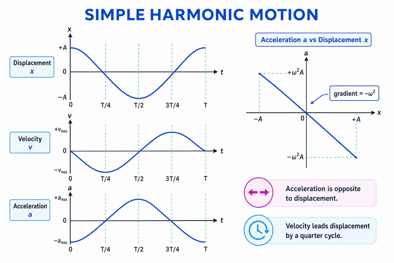
a=−ω2xa = -\omega^2 xa=−ω2xwhere aaa is acceleration in metres per second squared, xxx is displacement from equilibrium in metres, and ω\omegaω is the angular frequency in rad s^-1. The minus sign means the acceleration is always in the opposite direction to the displacement.
Because F=maF = maF=ma, the resultant force is also proportional to displacement and directed towards equilibrium.
Recognising SHM
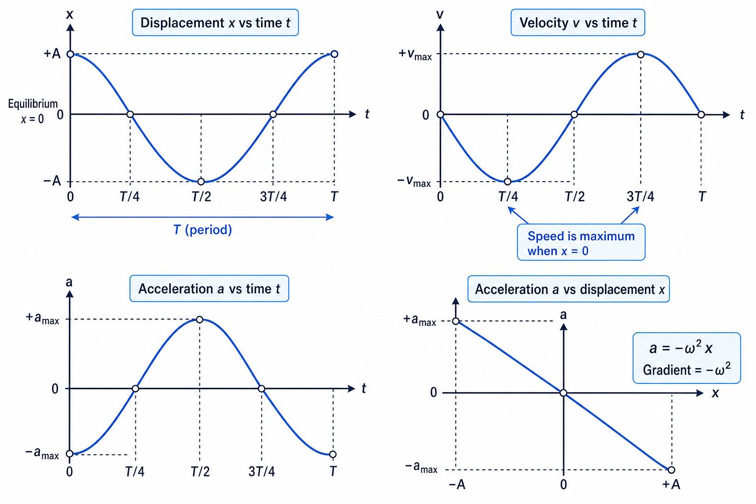
If a system has a∝−xa \propto -xa∝−x, it is undergoing simple harmonic motion. On an acceleration-displacement graph, SHM gives a straight line through the origin with negative gradient.
The graphs below show the key SHM relationships: acceleration is opposite to displacement, and the velocity graph is a quarter-cycle out of phase with displacement.
Using an acceleration-displacement graph
A mass has an acceleration-displacement graph that is a straight line through the origin with gradient −36 s−2-36\,\text{s}^{-2}−36s−2. Decide whether the motion is SHM and find the period.
-
A straight line through the origin with negative gradient means acceleration is proportional to displacement and acts in the opposite direction, so the motion is SHM.
-
Compare the graph gradient with a=−ω2xa = -\omega^2 xa=−ω2x. The gradient is −ω2-\omega^2−ω2, so:
ω2=36 s−2\omega^2 = 36\,\text{s}^{-2}ω2=36s−2 -
Take the square root:
ω=6.0 rad s−1\omega = 6.0\,\text{rad s}^{-1}ω=6.0rad s−1 -
Use T=2πωT = \frac{2\pi}{\omega}T=ω2π:
T=2π6.0 s−1=1.05 sT = \frac{2\pi}{6.0\,\text{s}^{-1}} = 1.05\,\text{s}T=6.0s−12π=1.05s
Amplitude, period, frequency and phase
The amplitude AAA is the maximum displacement from equilibrium, measured in metres.
The period TTT is the time for one complete oscillation, measured in seconds.
The frequency fff is the number of complete oscillations per second, measured in hertz.
The phase describes where an oscillator is in its cycle. One complete cycle corresponds to a phase change of 2π2\pi2π radians. The phase constant ε\varepsilonε sets the starting point of the motion at t=0t = 0t=0.
The relationships between period, frequency and angular frequency are:
T=1f=2πωT = \frac{1}{f} = \frac{2\pi}{\omega}T=f1=ω2πFor SHM, displacement can be written as:
x=Acos(ωt+ε)x = A \cos(\omega t + \varepsilon)x=Acos(ωt+ε)This is a solution to a=−ω2xa = -\omega^2 xa=−ω2x. Differentiating once gives the velocity:
v=−Aωsin(ωt+ε)v = -A\omega \sin(\omega t + \varepsilon)v=−Aωsin(ωt+ε)Differentiating again gives:
a=−Aω2cos(ωt+ε)a = -A\omega^2 \cos(\omega t + \varepsilon)a=−Aω2cos(ωt+ε)Since x=Acos(ωt+ε)x = A \cos(\omega t + \varepsilon)x=Acos(ωt+ε), this becomes a=−ω2xa = -\omega^2 xa=−ω2x.
At the centre, x=0x = 0x=0 and speed is maximum. At the extremes, x=±Ax = \pm Ax=±A and velocity is zero.
Maximum values
For SHM, the maximum speed is vmax=Aωv_\text{max} = A\omegavmax=Aω and the maximum acceleration is amax=Aω2a_\text{max} = A\omega^2amax=Aω2.
Calculator angle mode
When using x=Acos(ωt+ε)x = A\cos(\omega t + \varepsilon)x=Acos(ωt+ε) or v=−Aωsin(ωt+ε)v = -A\omega\sin(\omega t + \varepsilon)v=−Aωsin(ωt+ε), the angle ωt+ε\omega t + \varepsilonωt+ε is normally in radians if ω\omegaω is in rad s^-1.
Finding displacement and velocity
An oscillator has amplitude A=0.050 mA = 0.050\,\text{m}A=0.050m and frequency f=2.0 Hzf = 2.0\,\text{Hz}f=2.0Hz. It starts at maximum positive displacement, so ε=0\varepsilon = 0ε=0. Find xxx and vvv at t=0.10 st = 0.10\,\text{s}t=0.10s.
-
Find the angular frequency:
ω=2πf=2π(2.0 s−1)=12.6 rad s−1\omega = 2\pi f = 2\pi(2.0\,\text{s}^{-1}) = 12.6\,\text{rad s}^{-1}ω=2πf=2π(2.0s−1)=12.6rad s−1 -
Find the phase angle at this time:
ωt=(12.6 s−1)(0.10 s)=1.26 rad\omega t = (12.6\,\text{s}^{-1})(0.10\,\text{s}) = 1.26\,\text{rad}ωt=(12.6s−1)(0.10s)=1.26rad -
Substitute into the displacement equation:
x=(0.050 m)cos(1.26)=0.015 mx = (0.050\,\text{m})\cos(1.26) = 0.015\,\text{m}x=(0.050m)cos(1.26)=0.015m -
Substitute into the velocity equation:
v=−(0.050 m)(12.6 s−1)sin(1.26)=−0.60 m s−1v = -(0.050\,\text{m})(12.6\,\text{s}^{-1})\sin(1.26) = -0.60\,\text{m s}^{-1}v=−(0.050m)(12.6s−1)sin(1.26)=−0.60m s−1
Mass on a spring
The stiffness kkk of a spring is the force per unit extension, measured in newtons per metre.
For a mass mmm on a spring undergoing SHM:
T=2πmkT = 2\pi \sqrt{\frac{m}{k}}T=2πkmThis applies when the spring obeys Hooke’s law and damping is small. The period does not depend on amplitude, provided the oscillations are small enough for the spring to remain elastic.
Calculating a spring-mass period
A mass of 0.250 kg0.250\,\text{kg}0.250kg is attached to a spring of stiffness 18 N m−118\,\text{N m}^{-1}18N m−1. Find the period and frequency.
-
Substitute into the period equation:
T=2π0.250 kg18 N m−1T = 2\pi \sqrt{\frac{0.250\,\text{kg}}{18\,\text{N m}^{-1}}}T=2π18N m−10.250kg -
Check the unit behaviour: since 1 N=1 kg m s−21\,\text{N} = 1\,\text{kg m s}^{-2}1N=1kg m s−2, the quantity inside the square root has units of seconds squared.
-
Calculate the period:
T=0.740 sT = 0.740\,\text{s}T=0.740s -
Use f=1Tf = \frac{1}{T}f=T1:
f=10.740 s=1.35 Hzf = \frac{1}{0.740\,\text{s}} = 1.35\,\text{Hz}f=0.740s1=1.35Hz
Simple pendulum and measuring g
A simple pendulum is a small mass suspended from a light string, oscillating through a small angle. For small angles:
T=2πlgT = 2\pi \sqrt{\frac{l}{g}}T=2πglwhere lll is the length from the pivot to the centre of the bob, and ggg is the gravitational field strength.
Small-angle condition
The pendulum equation is only accurate for small oscillations, typically less than about 10 degrees. At larger angles, the motion is not close enough to ideal SHM.
Practical: measuring g with a pendulum
To measure ggg, you can rearrange the pendulum equation into a straight-line graph form:
T2=4π2glT^2 = \frac{4\pi^2}{g}lT2=g4π2lSo a graph of T2T^2T2 against lll should be a straight line through the origin with gradient:
gradient=4π2g\text{gradient} = \frac{4\pi^2}{g}gradient=g4π2A good method is to measure the length from pivot to centre of the bob, displace the bob by a small angle, and time 10 or 20 complete oscillations. Use a fiducial marker to judge the same point in each swing, repeat timings, then calculate the mean period using T=tNT = \frac{t}{N}T=Nt.
To improve reliability, use several different lengths, plot T2T^2T2 against lll, and find the gradient from a best-fit line. Timing many oscillations reduces the percentage uncertainty caused by reaction time.
Finding g from a pendulum graph
A graph of T2T^2T2 against lll has gradient 4.05 s2m−14.05\,\text{s}^2\text{m}^{-1}4.05s2m−1 with uncertainty 0.12 s2m−10.12\,\text{s}^2\text{m}^{-1}0.12s2m−1. Find ggg and its uncertainty.
-
Use the gradient relationship:
gradient=4π2g\text{gradient} = \frac{4\pi^2}{g}gradient=g4π2 -
Rearrange for ggg:
g=4π2gradientg = \frac{4\pi^2}{\text{gradient}}g=gradient4π2 -
Substitute the gradient:
g=4π24.05 s2m−1=9.75 m s−2g = \frac{4\pi^2}{4.05\,\text{s}^2\text{m}^{-1}} = 9.75\,\text{m s}^{-2}g=4.05s2m−14π2=9.75m s−2 -
Since ggg is inversely proportional to the gradient, the fractional uncertainty is the same:
Δgg=0.124.05=0.0296\frac{\Delta g}{g} = \frac{0.12}{4.05} = 0.0296gΔg=4.050.12=0.0296 -
Calculate the absolute uncertainty:
Δg=0.0296(9.75 m s−2)=0.29 m s−2\Delta g = 0.0296(9.75\,\text{m s}^{-2}) = 0.29\,\text{m s}^{-2}Δg=0.0296(9.75m s−2)=0.29m s−2
Energy changes in undamped SHM
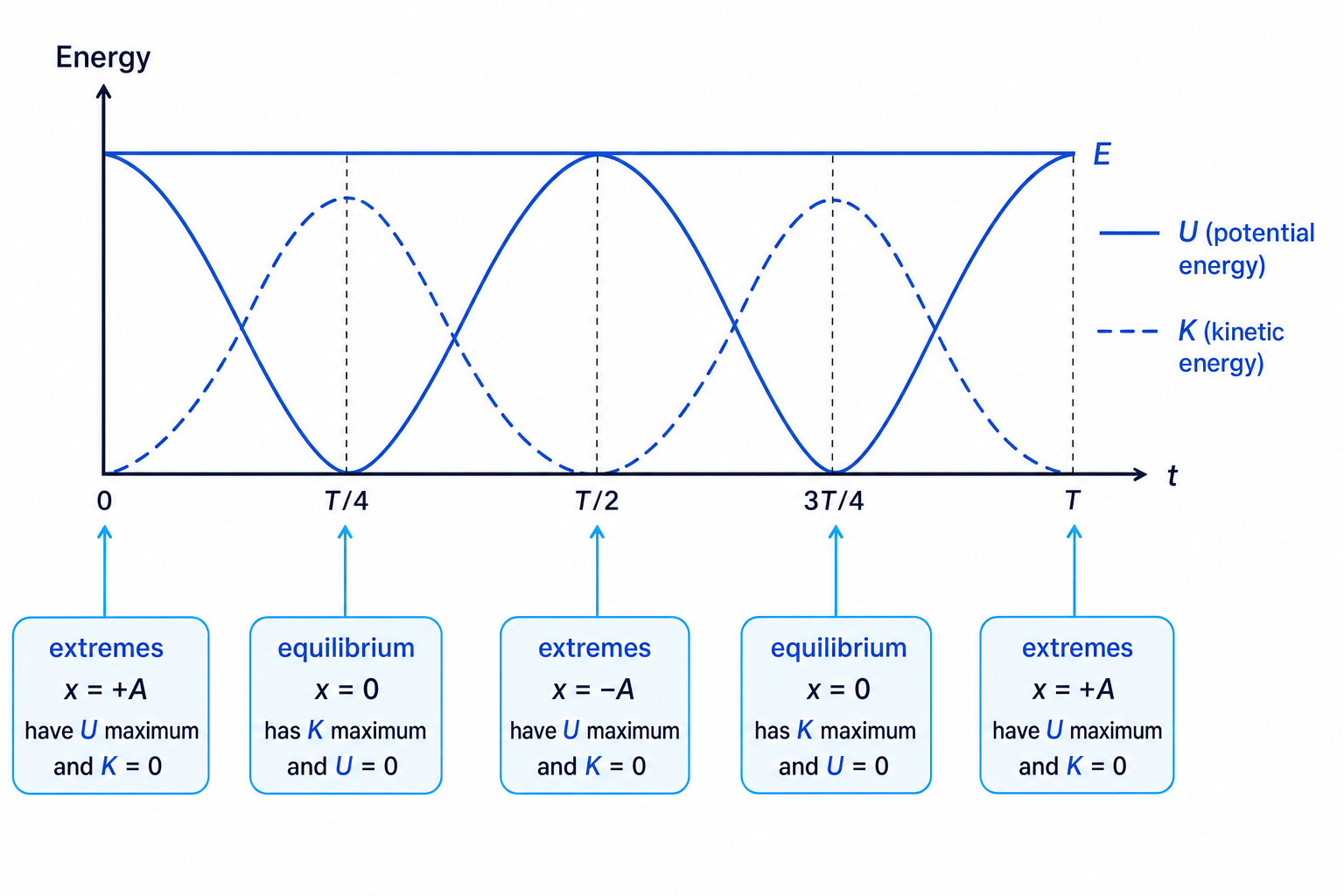
In undamped SHM, no energy is transferred to the surroundings, so the total mechanical energy stays constant.
Energy continually swaps between kinetic energy and potential energy. At maximum displacement, the oscillator is momentarily at rest, so kinetic energy is zero and potential energy is maximum. At equilibrium, speed is maximum, so kinetic energy is maximum and potential energy is minimum.
The graph below shows how kinetic energy and potential energy interchange while total energy remains constant.
For a spring oscillator measured from equilibrium:
Etotal=12kA2E_\text{total} = \frac{1}{2}kA^2Etotal=21kA2and at displacement xxx:
Ep=12kx2E_p = \frac{1}{2}kx^2Ep=21kx2so:
Ek=Etotal−EpE_k = E_\text{total} - E_pEk=Etotal−EpCalculating energy and speed
A 0.50 kg0.50\,\text{kg}0.50kg mass oscillates on a spring of stiffness 20 N m−120\,\text{N m}^{-1}20N m−1 with amplitude 0.080 m0.080\,\text{m}0.080m. Find the kinetic energy and speed when x=0.030 mx = 0.030\,\text{m}x=0.030m.
-
Calculate the total energy:
Etotal=12(20 N m−1)(0.080 m)2=0.064 JE_\text{total} = \frac{1}{2}(20\,\text{N m}^{-1})(0.080\,\text{m})^2 = 0.064\,\text{J}Etotal=21(20N m−1)(0.080m)2=0.064J -
Calculate the potential energy at x=0.030 mx = 0.030\,\text{m}x=0.030m:
Ep=12(20 N m−1)(0.030 m)2=0.0090 JE_p = \frac{1}{2}(20\,\text{N m}^{-1})(0.030\,\text{m})^2 = 0.0090\,\text{J}Ep=21(20N m−1)(0.030m)2=0.0090J -
Use conservation of energy:
Ek=0.064 J−0.0090 J=0.055 JE_k = 0.064\,\text{J} - 0.0090\,\text{J} = 0.055\,\text{J}Ek=0.064J−0.0090J=0.055J -
Use Ek=12mv2E_k = \frac{1}{2}mv^2Ek=21mv2:
v=2Ekm=2(0.055 J)0.50 kg=0.47 m s−1v = \sqrt{\frac{2E_k}{m}} = \sqrt{\frac{2(0.055\,\text{J})}{0.50\,\text{kg}}} = 0.47\,\text{m s}^{-1}v=m2Ek=0.50kg2(0.055J)=0.47m s−1
Free oscillations and damping
A free oscillation occurs when a system is displaced and released, then oscillates at its own natural frequency without a continuous external driving force.
Damping is the loss of mechanical energy from an oscillating system, usually due to resistive forces such as air resistance or friction. The amplitude decreases with time because energy is transferred to the surroundings, often as internal energy and sound.
Practical examples of damped oscillations include a pendulum slowing down in air, a mass on a spring in oil, a door closer, a seismometer, and a car suspension system.
Practical: investigating damping of a spring
You can investigate damping by hanging a mass from a spring, displacing it by a fixed amplitude, and recording how the peak amplitude changes with time. Damping can be changed by attaching a card to the mass, placing the mass in water or oil, or using different surrounding fluids.
Useful measurement methods include a ruler with a fiducial marker, video analysis, or a motion sensor. Repeat the experiment for each damping condition and keep the initial displacement the same. A graph of amplitude against time lets you compare how quickly the oscillations die away.
Uncertainty in damping experiments
Use the same reference point for every amplitude reading, avoid parallax by viewing the scale square-on, and repeat runs because the release technique can noticeably affect the first few oscillations.
Critical damping
A system is critically damped when it returns to equilibrium in the shortest possible time without oscillating.
This is important in vehicle suspensions. After a car goes over a bump, you want the body of the car to return smoothly to its normal position without bouncing repeatedly. Too little damping gives uncomfortable oscillations; too much damping makes the suspension slow to respond.
Why critical damping matters
Critical damping removes oscillations quickly without overshooting repeatedly, so it is useful when stability and a fast return to equilibrium are both needed.
Forced oscillations and resonance
A forced oscillation happens when an external periodic force drives a system. The frequency of this external force is the driving frequency.
Resonance occurs when the driving frequency is close to the natural frequency of the system. The amplitude becomes large because energy is transferred efficiently from the driver to the oscillator.
The graph below shows how amplitude varies with driving frequency, and how damping affects the resonance curve.
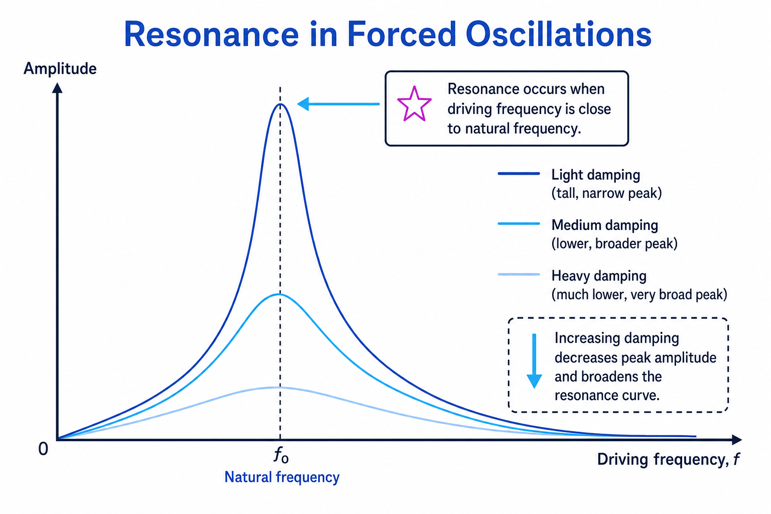
With light damping, the resonance peak is tall and narrow. Increasing damping decreases the maximum amplitude and broadens the resonance curve, so the system responds less violently over a wider range of frequencies.
Interpreting a resonance risk
A footbridge has a natural frequency close to the stepping frequency of pedestrians. Explain the risk and how engineers could reduce it.
-
If the stepping frequency is close to the bridge’s natural frequency, the bridge undergoes forced oscillations near resonance.
-
At resonance, energy is transferred efficiently into the bridge each cycle, so the amplitude of vibration can become large if damping is low.
-
Engineers can reduce the risk by increasing damping, changing the bridge’s stiffness or mass to shift its natural frequency, or preventing pedestrians from walking in step.
Resonance can be useful. In circuit tuning, a circuit is adjusted so its natural frequency matches the frequency of the desired radio signal. In microwave cooking, the oscillating electric field transfers energy effectively to water molecules in food. Musical instruments also use resonance to amplify selected frequencies.
Resonance can also be dangerous. It should be avoided in bridge design, tall buildings, rotating machinery and vehicle components. Designers often add damping or choose dimensions and materials so the natural frequency is well away from likely driving frequencies.
In the exam
-
For SHM questions, start from a=−ω2xa = -\omega^2 xa=−ω2x: a negative straight-line acceleration-displacement graph is the giveaway.
-
In calculation questions, measure displacement from equilibrium, use radians with ωt\omega tωt, and carry units through every substitution.
-
For practical questions, mention timing many oscillations, repeating readings, plotting a straight-line graph, using the gradient, and reducing uncertainty with careful measurement.
Check yourself
-
If an acceleration-displacement graph has gradient −25 s−2-25\,\text{s}^{-2}−25s−2, what are ω\omegaω and TTT?
-
Why does the pendulum method use small angles and time many oscillations rather than just one?
-
How does increased damping change the resonance curve, and why is that useful in a car suspension?