

What you'll learn
- How progressive waves transfer energy without transferring matter overall.
- How to distinguish transverse and longitudinal waves.
- How to use displacement, amplitude, wavelength, frequency, period and wave velocity.
- How polarisation, phase, wavefronts and rays are described and tested experimentally.
1. Waves begin with oscillations
An oscillation is a repeated motion about an equilibrium position. The equilibrium position is the undisturbed position a particle would have if no wave were passing.
A wave can travel through a medium, meaning the material or substance through which the wave passes, such as air, water or a stretched string. Electromagnetic waves do not need a material medium.
Progressive wave
A progressive wave is a disturbance that travels from one place to another, transferring energy without any overall transfer of matter.
For example, particles in a rope move up and down as the wave passes, but they do not travel along the rope with the wave. The wave pattern and energy move along; the rope particles only oscillate locally.
Energy, not matter
In a progressive wave, energy is transferred in the direction of wave travel, while the particles of the medium oscillate about fixed equilibrium positions.
2. Transverse and longitudinal waves
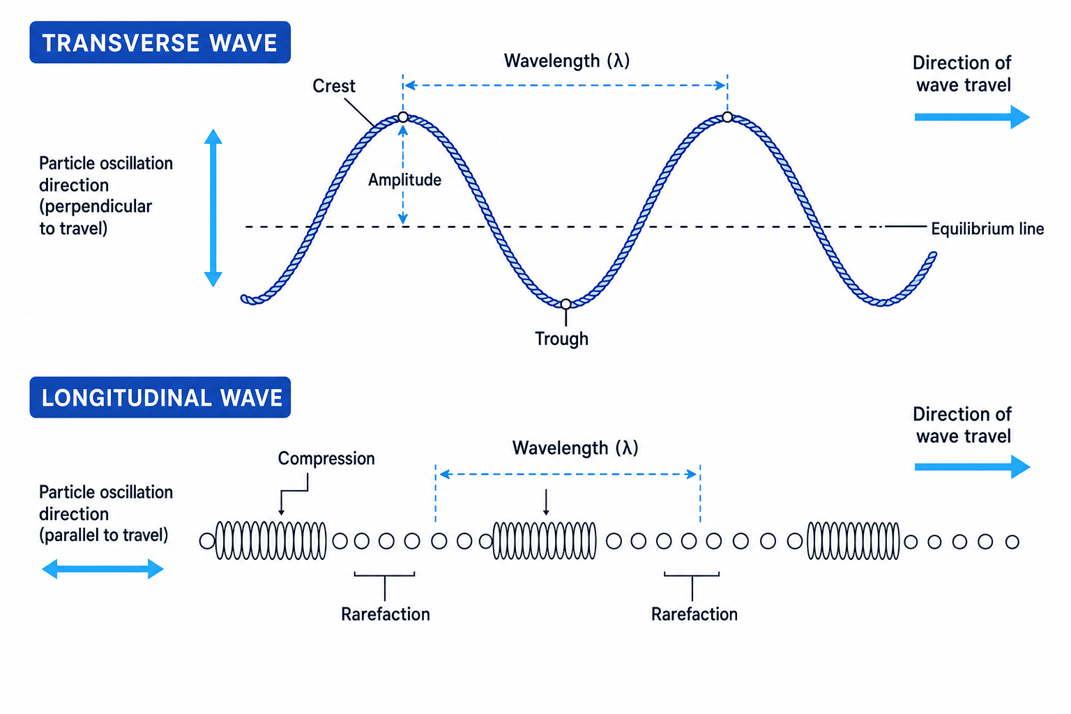
The key difference is the direction of the oscillations compared with the direction in which energy is transferred.
Transverse and longitudinal waves
- In a transverse wave, the oscillations are perpendicular to the direction of wave travel.
- In a longitudinal wave, the oscillations are parallel to the direction of wave travel.
Examples of transverse waves include electromagnetic waves and waves on a stretched string. Examples of longitudinal waves include sound waves in air and compression waves in a spring.
In a longitudinal wave, a compression is a region where particles are closer together than normal. A rarefaction is a region where particles are further apart than normal.
Particle motion is not wave motion
Do not say that the particles travel all the way from source to detector. In a progressive wave, particles oscillate locally; the disturbance and energy travel through the medium.
3. The language of wave measurements
You need to be fluent with these quantities before using the wave equation.
Wave quantities
- Displacement is the distance and direction of a point on the wave from its equilibrium position. It is measured in metres, m.
- Amplitude, AAA, is the maximum displacement from equilibrium. It is measured in metres, m.
- Wavelength, λ\lambdaλ, is the distance between adjacent points that are in phase, such as crest to crest or compression to compression. It is measured in metres, m.
- Frequency, fff, is the number of complete oscillations per second. It is measured in hertz, Hz.
- Period, TTT, is the time for one complete oscillation. It is measured in seconds, s, and f=1Tf=\frac{1}{T}f=T1.
- Wave velocity or wave speed, ccc, is the speed at which the wave pattern or wavefront travels. It is measured in metres per second, m s⁻¹.
During one period, the wave travels one wavelength. So:
c=fλc=f\lambdac=fλYou should also be able to rearrange it:
f=cλλ=cff=\frac{c}{\lambda} \qquad \lambda=\frac{c}{f}f=λcλ=fcUnit conversions first
Before using c=fλc=f\lambdac=fλ, convert all distances to metres and all frequencies to hertz. For example, 2.45 GHz=2.45×10⁹ Hz2.45\ \text{GHz}=2.45\times10^9\ \text{Hz}2.45 GHz=2.45×10⁹ Hz.
4. Displacement graphs and wavefronts
For this specification, displacement-position graphs are treated for transverse waves only.
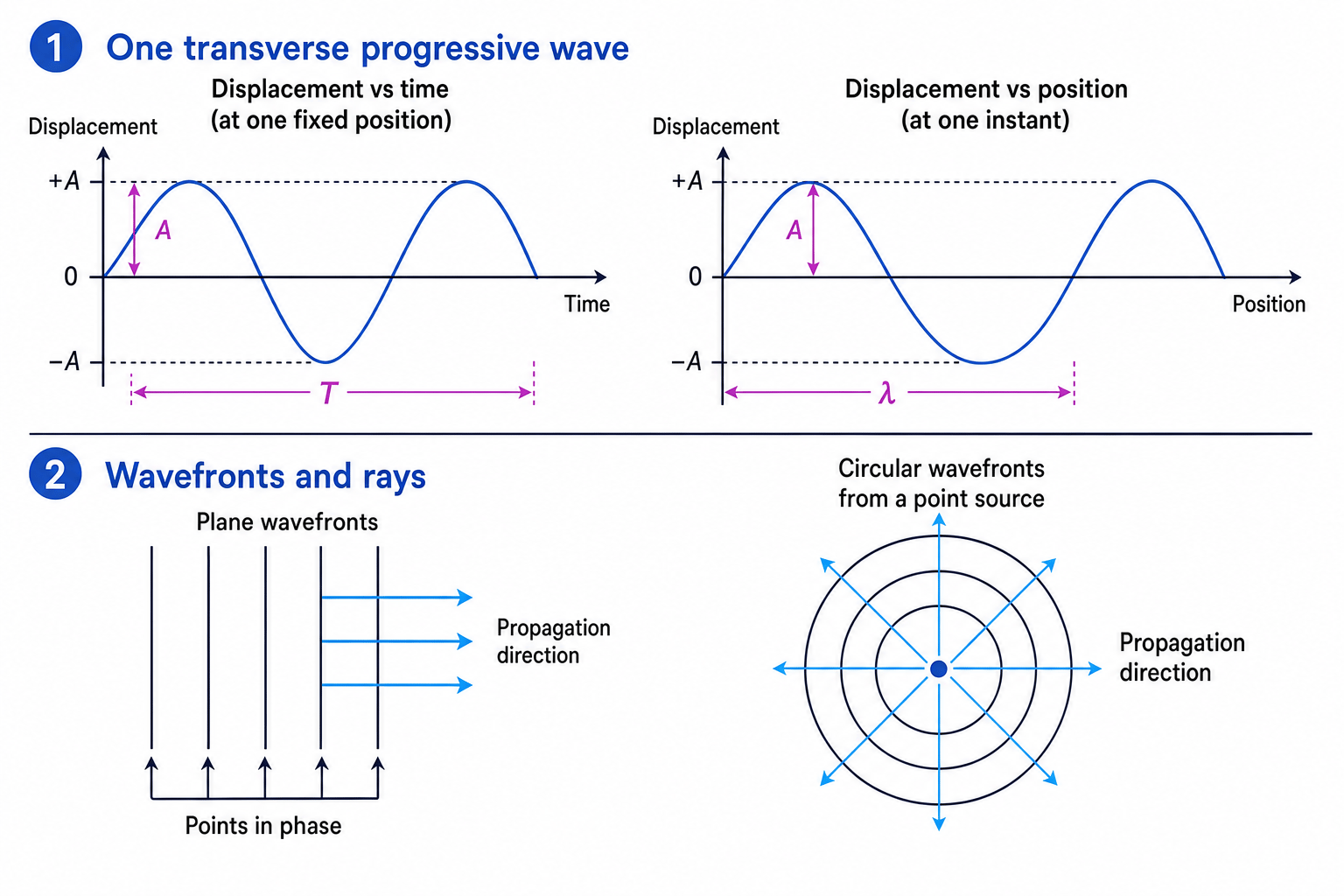
A displacement-time graph shows how one point on the wave oscillates as time passes. A displacement-position graph shows the shape of the wave along its length at one instant.
A wavefront is a line or surface joining points that oscillate in phase. A ray is an arrow showing the direction of wave propagation. Rays are always at right angles to wavefronts.
Using graph readings to find wave speed
-
From a displacement-time graph, adjacent crests occur at 0.15 s and 0.55 s, so the period is
T=0.55 s−0.15 s=0.40 sT=0.55\ \text{s}-0.15\ \text{s}=0.40\ \text{s}T=0.55 s−0.15 s=0.40 s. -
Calculate the frequency using f=1Tf=\frac{1}{T}f=T1:
f=10.40 s=2.5 Hzf=\frac{1}{0.40\ \text{s}}=2.5\ \text{Hz}f=0.40 s1=2.5 Hz. -
From a displacement-position graph, adjacent crests occur at 0.20 m and 1.00 m, so the wavelength is
λ=1.00 m−0.20 m=0.80 m\lambda=1.00\ \text{m}-0.20\ \text{m}=0.80\ \text{m}λ=1.00 m−0.20 m=0.80 m. -
Use the wave equation:
c=fλ=2.5 Hz×0.80 m=2.0 m s−1c=f\lambda=2.5\ \text{Hz}\times0.80\ \text{m}=2.0\ \text{m s}^{-1}c=fλ=2.5 Hz×0.80 m=2.0 m s−1.
Mixing up the two graph axes
On a displacement-time graph, the horizontal spacing gives the period. On a displacement-position graph, the horizontal spacing gives the wavelength.
5. Phase, in phase and antiphase
Phase describes where an oscillating point is in its cycle.
Two points are in phase if they are at the same point in their oscillation at the same time: same displacement and moving in the same direction. Their phase difference is a whole number of cycles.
Two points are in antiphase if they are half a cycle apart. When one has maximum positive displacement, the other has maximum negative displacement.
In phase and antiphase
- Points separated by a whole number of wavelengths are in phase.
- Points separated by an odd number of half-wavelengths are in antiphase.
- In radians, antiphase corresponds to a phase difference of π\piπ radians.
Deciding the phase relationship
-
Two points on a wave are separated by 0.96 m, and the wavelength is 0.64 m. Compare the separation with the wavelength:
Δxλ=0.96 m0.64 m=1.5\frac{\Delta x}{\lambda}=\frac{0.96\ \text{m}}{0.64\ \text{m}}=1.5λΔx=0.64 m0.96 m=1.5. -
A separation of 1.5 wavelengths is one whole wavelength plus half a wavelength, so the points are half a cycle out after allowing for the full cycle.
-
Therefore the two points are in antiphase.
6. Polarisation
Polarisation is a property of transverse waves.
Polarisation
Polarisation is the restriction of wave oscillations to one plane or direction.
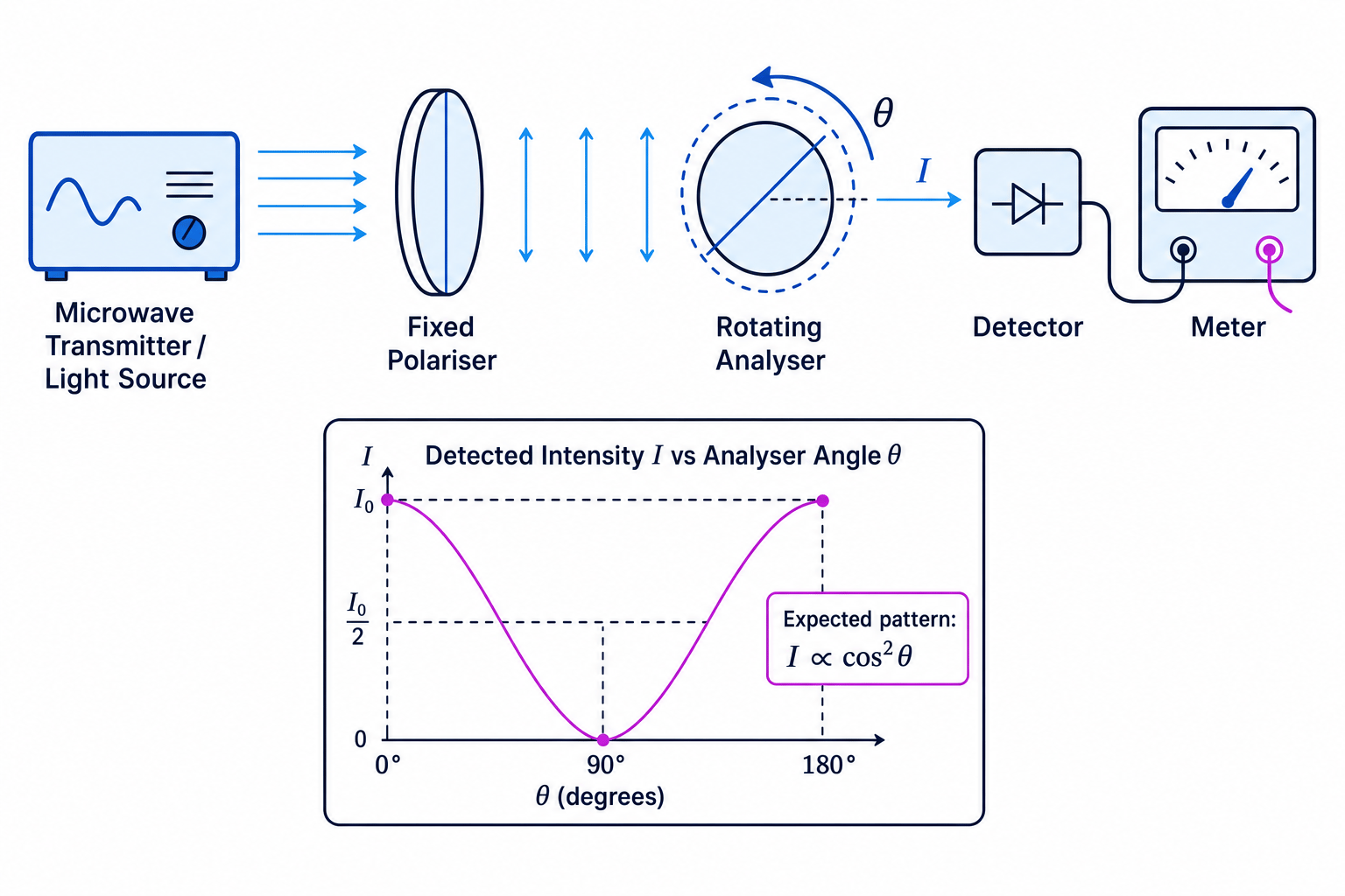
For an electromagnetic wave, the oscillating electric field can be restricted to one direction. A polariser produces a polarised wave. A second polariser used to test the polarisation is often called an analyser.
Longitudinal waves cannot be polarised because their oscillations are only along the direction of travel; there is no sideways oscillation direction to restrict.
Polarisation test
If a wave can be polarised, it must be transverse. This is strong evidence that electromagnetic waves are transverse waves.
7. Specified practical: intensity variations for polarisation
In this practical, intensity means the received wave power per unit area. In school apparatus, a detector voltage or current is often used as a quantity proportional to intensity.
Method
- Align the microwave transmitter or light source, polariser, analyser and detector so that the detector reading is initially large.
- Keep the source-detector distance fixed throughout.
- Define the analyser angle θ\thetaθ relative to the polariser’s transmission axis.
- Rotate the analyser from 0° to 180° in equal intervals, such as 10° or 15°.
- Record the detector reading at each angle. Repeat readings and calculate a mean.
- Plot mean detector reading against analyser angle θ\thetaθ.
For ideal plane-polarised radiation, the intensity follows:
I=I0cos2θI=I_0\cos^2\thetaI=I0cos2θSo maxima occur when the polariser and analyser axes are parallel, and a minimum occurs when they are at 90°.
Checking polarisation data
-
Calculate the mean maximum reading at 0°:
Iˉ0=(4.8+4.9+4.7) mV3=4.8 mV\bar I_0=\frac{(4.8+4.9+4.7)\ \text{mV}}{3}=4.8\ \text{mV}Iˉ0=3(4.8+4.9+4.7) mV=4.8 mV. -
Calculate the mean reading at 60°:
Iˉ60=(1.1+1.2+1.3) mV3=1.2 mV\bar I_{60}=\frac{(1.1+1.2+1.3)\ \text{mV}}{3}=1.2\ \text{mV}Iˉ60=3(1.1+1.2+1.3) mV=1.2 mV. -
Compare the measured fraction with the maximum:
Iˉ60Iˉ0=1.2 mV4.8 mV=0.25\frac{\bar I_{60}}{\bar I_0}=\frac{1.2\ \text{mV}}{4.8\ \text{mV}}=0.25Iˉ0Iˉ60=4.8 mV1.2 mV=0.25. -
Compare with the expected value:
cos260∘=0.25\cos^2 60^\circ=0.25cos260∘=0.25, so the data are consistent with the expected polarisation pattern.
Practical quality and evaluation
Use repeat readings to reduce random uncertainty, and quote meter readings to the resolution of the instrument. If the reading at 90° is not zero, possible reasons include background radiation, imperfect polarisers, detector offset, misalignment, or reflections from nearby surfaces.
Testing the model
A plot of III against cos2θ\cos^2\thetacos2θ should be a straight line for ideal polarisation. A non-zero intercept suggests a background or zero error.
Transmission axis confusion
For microwave grids, do not guess the transmission axis from the visible wires unless the apparatus instructions state it. Use the marked polarisation direction or determine it experimentally.
In the exam
- For wave graphs, identify the axis first: time spacing gives TTT, position spacing gives λ\lambdaλ.
- For c=fλc=f\lambdac=fλ, convert prefixes before substituting, especially kHz, MHz, GHz, cm and mm.
- For polarisation practical questions, describe both the pattern of results and the quality of the method: repeats, fixed distance, angle uncertainty, background readings and alignment.
Check yourself
- How can a wave transfer energy without transferring matter overall?
- What observation would show that a wave is transverse rather than longitudinal?
- On a displacement-time graph, how would you find the frequency of the wave?
