

What you'll learn
- The difference between a high-frequency carrier wave and a low-frequency information signal.
- How Amplitude Modulation (AM) and Frequency Modulation (FM) work, and how to interpret their graphs.
- How to calculate the carrier frequency and information frequency from a voltage-time graph.
- How to calculate the bandwidth requirements for AM and FM transmissions.
- How bandwidth availability affects the data capacity of different communication media.
1. The Principles of Modulation
To transmit an audio or data signal over long distances (like radio broadcasting), we run into a major physical problem. Human speech and music are low-frequency sound waves, usually ranging from 20 Hz20 \text{ Hz}20 Hz to 20 kHz20 \text{ kHz}20 kHz. If we simply converted these sound waves into electrical signals and tried to transmit them as electromagnetic radio waves, we would need transmission antennas several kilometres long!
To solve this, we use a technique called modulation.
Modulation
Modulation is the process of altering a specific characteristic (such as amplitude or frequency) of a high-frequency continuous wave so that it can carry a lower-frequency data signal.
There are two main signals involved in this process:
- The Information Signal: This is the data you actually want to send (e.g., voice, music, or digital data). It is typically a low-frequency, low-energy signal.
- The Carrier Wave: This is a high-frequency, constant-amplitude electromagnetic wave. It does not carry any useful information on its own, but its high frequency allows it to be transmitted efficiently through the air using reasonably sized antennas.
By combining the two, the information signal "rides" on the carrier wave.
2. Amplitude Modulation (AM)
In Amplitude Modulation, the frequency of the carrier wave is kept completely constant, but its amplitude is continuously varied in proportion to the displacement of the information signal.
When the information signal's voltage is high, the carrier wave's amplitude increases. When the information signal's voltage is low or negative, the carrier wave's amplitude decreases.
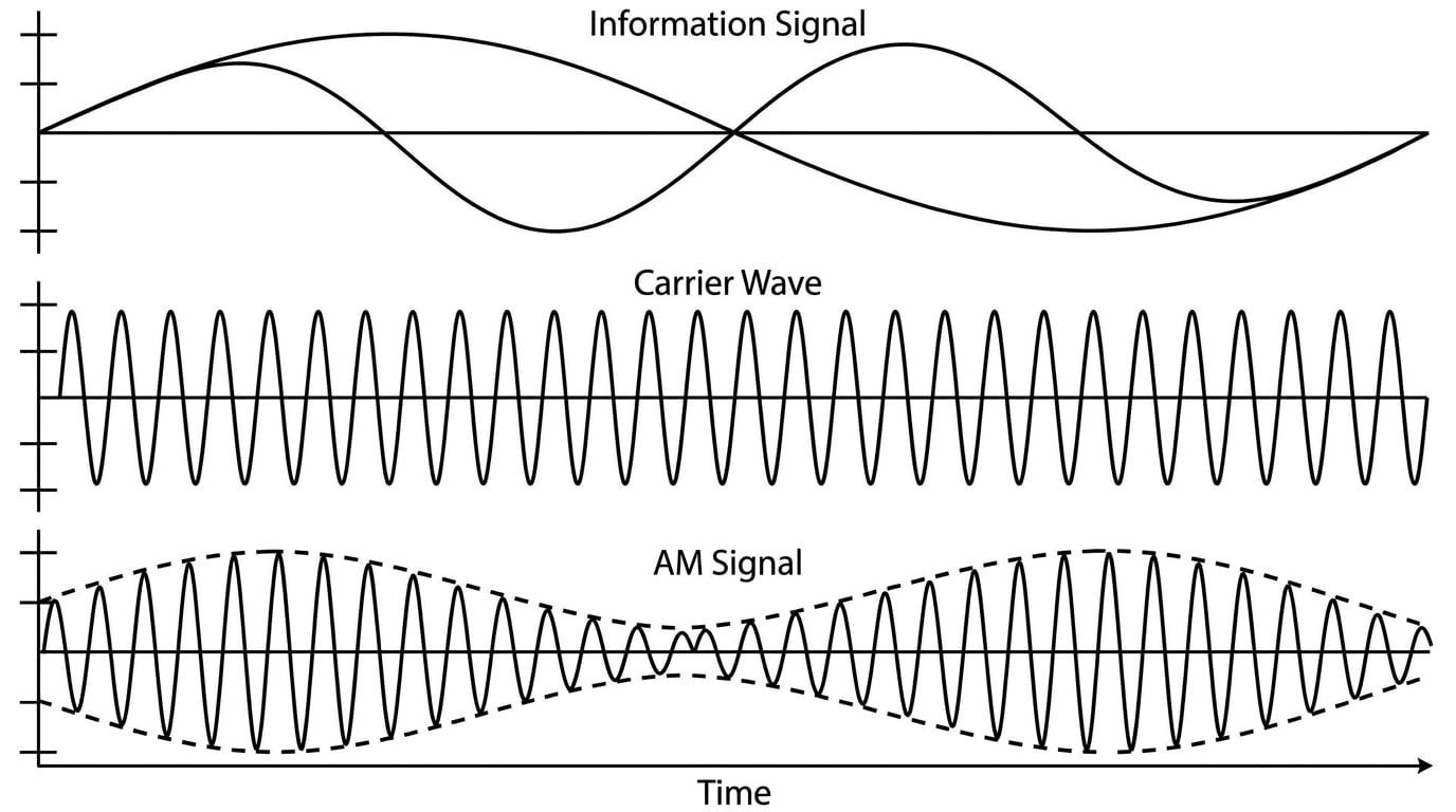
Notice the outer boundary of the modulated AM signal in the bottom graph. This shape perfectly traces the original low-frequency information signal and is known as the envelope.
Reading AM Graphs
An AM signal graph contains both frequencies:
- The information frequency (fMf_MfM) is found by looking at the slow, repeating pattern of the envelope.
- The carrier frequency (fcf_cfc) is found by looking at the fast, highly compressed individual waves inside the envelope.
Finding frequencies from an AM trace
An oscilloscope displays an AM signal. The time base is set so that the total width of the screen represents 10 ms10 \text{ ms}10 ms. Across the full screen, there are exactly 444 complete cycles of the overall envelope. Zooming in reveals that inside one complete envelope cycle, there are 505050 individual high-frequency oscillations.
Calculate the information frequency (fMf_MfM) and the carrier frequency (fcf_cfc).
- Find the time period of the information signal (TMT_MTM): There are 444 envelope cycles in 10 ms10 \text{ ms}10 ms.
- Calculate the information frequency (fMf_MfM):
- Find the time period of the carrier wave (TcT_cTc): One envelope cycle takes 2.5 ms2.5 \text{ ms}2.5 ms. We are told there are 505050 carrier oscillations in this single envelope cycle.
- Calculate the carrier frequency (fcf_cfc):
Counting half-cycles
When counting envelope cycles to find the information frequency, be careful not to confuse the top half of the envelope with a full wave. A single complete cycle of the information signal goes from a peak amplitude, down to a minimum amplitude, and back up to a peak.
3. Frequency Modulation (FM)
In Frequency Modulation, the amplitude of the carrier wave remains completely constant. Instead, the frequency of the carrier wave is varied in proportion to the voltage of the information signal.
- When the information signal is at a high positive voltage, the carrier frequency increases (the waves bunch tightly together).
- When the information signal is at a negative voltage, the carrier frequency decreases (the waves spread further apart).
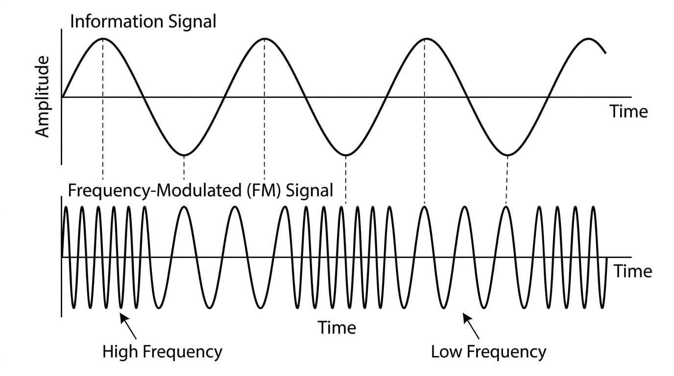
In FM, the loudest parts of an audio signal (highest amplitude) cause the greatest change in the carrier's frequency. This maximum shift away from the resting carrier frequency is called the frequency deviation, denoted by the symbol Δf\Delta fΔf.
Why use FM?
Because FM relies on frequency changes rather than amplitude changes, it is much less susceptible to electrical interference and static. Lightning or heavy machinery often causes random spikes in a radio wave's amplitude (which ruins AM audio), but this "noise" doesn't change the wave's frequency, leaving FM signals crystal clear.
4. Bandwidth Requirements
When a carrier wave is modulated, it doesn't just occupy a single frequency anymore. The modulation process generates additional frequencies around the original carrier frequency.
Bandwidth
Bandwidth is the total range of frequencies that a transmission occupies. It is the difference between the highest and lowest frequencies present in the modulated signal.
The AQA specification requires you to know how to calculate the bandwidth for both simple AM and FM transmissions.
Bandwidth of an AM Signal
For Amplitude Modulation, the bandwidth is exactly twice the maximum frequency of the information signal (fMf_MfM).
AM Bandwidth=2fM \text{AM Bandwidth} = 2f_M AM Bandwidth=2fMBandwidth of an FM Signal
For Frequency Modulation, the calculation uses Carson's Rule. It depends on both the maximum frequency of the information signal (fMf_MfM) and the maximum frequency deviation (Δf\Delta fΔf).
FM Bandwidth=2(Δf+fM) \text{FM Bandwidth} = 2(\Delta f + f_M) FM Bandwidth=2(Δf+fM)Calculating Bandwidth
A local radio station wants to broadcast high-fidelity music containing audio frequencies up to 15 kHz15 \text{ kHz}15 kHz. a) Calculate the bandwidth required if they broadcast using AM. b) Calculate the bandwidth required if they broadcast using FM, assuming a maximum frequency deviation of 75 kHz75 \text{ kHz}75 kHz.
Part a) AM Bandwidth:
- Identify the highest information frequency (fMf_MfM):
- Apply the AM formula:
Part b) FM Bandwidth:
- Identify the variables:
- Apply the FM formula:
Notice how much more bandwidth FM requires compared to AM! This is why FM radio stations are spaced much further apart on your radio dial than AM stations.
5. Data Capacity and Transmission Media
The concept of bandwidth isn't just about radio stations—it is the most important factor in modern data communications, like your home broadband.
Data capacity is the maximum rate at which information can be transmitted over a communication channel (measured in bits per second).
There is a direct relationship between bandwidth and data capacity: the wider the bandwidth of a channel, the higher its data capacity. If you want to download games faster or stream 4K video, your physical connection needs a wider bandwidth.
Different physical media can support very different bandwidths:
- Twisted Pair Copper Wires (e.g., old telephone lines): These suffer from high attenuation and interference at high frequencies. They have a very narrow bandwidth, making them suitable only for low-capacity voice calls or slow ADSL broadband.
- Coaxial Cables (e.g., TV aerials, Virgin Media broadband): Because the inner wire is shielded by an outer conductive mesh, they can carry much higher frequencies without losing the signal to interference. They have a medium-to-high bandwidth and can carry hundreds of TV channels or fast broadband.
- Optical Fibres: Because they use visible or infrared light (which has an incredibly high frequency of roughly 1014 Hz10^{14} \text{ Hz}1014 Hz), optical fibres can offer a phenomenal bandwidth. Their data capacity is practically limitless, allowing gigabits or even terabits of data to be transmitted per second.
Bandwidth as a motorway
Think of bandwidth like the number of lanes on a motorway. A twisted copper pair is a single-lane country road—only a few cars (bits of data) can pass per second. An optical fibre is a massive 50-lane superhighway where enormous volumes of traffic can flow smoothly at the same time.
In the exam
- Check your prefixes: Be extremely careful reading graphs or text containing prefixes. Milliseconds (ms\text{ms}ms, 10−310^{-3}10−3) and microseconds (μs\mu\text{s}μs, 10−610^{-6}10−6) are very common in AQA oscilloscope questions. Convert to seconds immediately before calculating frequency.
- Use average values for graphs: If asked to calculate a frequency from a graph, do not measure the time for just one small cycle. Measure the total time for as many full cycles as you can see, then divide by the number of cycles to find the time period TTT. This minimises your reading error.
- Remember the brackets: In the FM bandwidth formula, remember that the addition (Δf+fM)(\Delta f + f_M)(Δf+fM) happens before you multiply by 2.
Check yourself
- What visual feature of an AM graph allows you to determine the information signal's frequency?
- In an FM signal, what happens to the carrier wave when the information signal reaches a deep trough (large negative voltage)?
- If an FM transmitter uses a maximum deviation of 50 kHz50 \text{ kHz}50 kHz to send a 10 kHz10 \text{ kHz}10 kHz audio signal, what total bandwidth is required?
- Why do optical fibres have a vastly greater data capacity than twisted copper pairs?
