2.5.1a Fiscal policy and its functions
Fiscal Policy Uses Spending, Taxation and the Budget Balance to Steer the Economy
Fiscal policy: the use of government spending, taxation and the budget balance to influence aggregate demand, aggregate supply and the pattern of economic activity.
- Fiscal policy uses government spending, taxation and the budget balance to influence the economy.
- In the UK it is set by HM Treasury and announced by the Chancellor in the annual Budget.
- Expansionary fiscal policy raises spending or cuts taxes to lift aggregate demand.
- Contractionary fiscal policy cuts spending or raises taxes to slow it.
Three Functions: Demand-Side, Supply-Side and Microeconomic
- Fiscal policy works mainly on the demand side, but it also has supply-side and microeconomic effects.
- Demand-side: changes in spending and taxation shift aggregate demand, affecting output, employment and the price level.
- Supply-side: tax changes alter incentives to work and invest, and spending on skills or infrastructure raises productive capacity.
- Microeconomic: government spending and taxation change the pattern of economic activity, affecting households, firms and particular markets differently.
Showing Fiscal Policy on an AD/AS Diagram
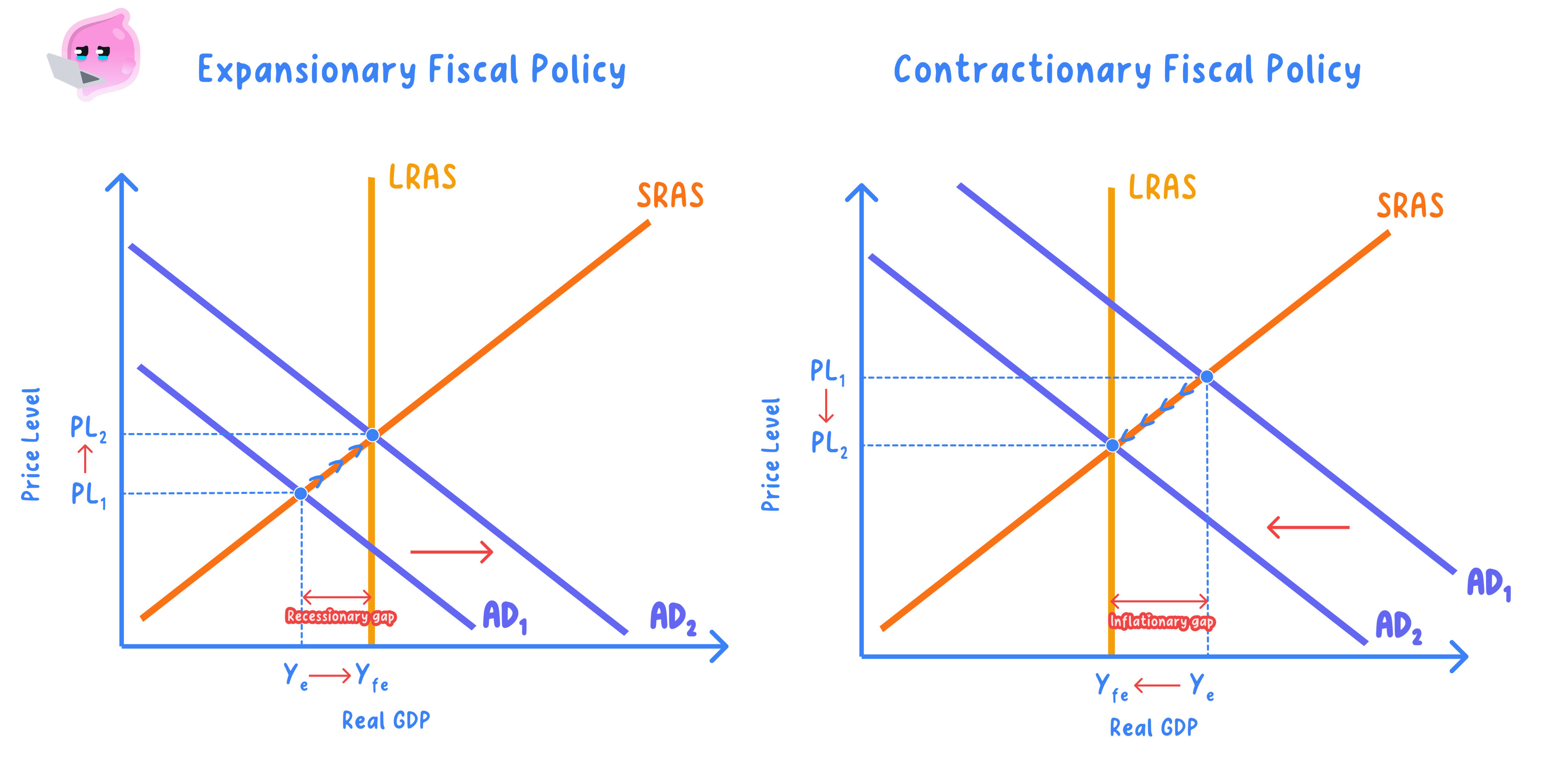
- Label the axes as the average price level and real output.
- Expansionary policy shifts aggregate demand to the right, raising real output, the price level and employment; contractionary policy shifts it to the left.
- How far output rises rather than the price level depends on the slope of the AS curve and how close the economy is to full capacity.
How Effective Is Fiscal Policy?
- Time lags: recognition, decision and impact lags can mean the policy arrives too late.
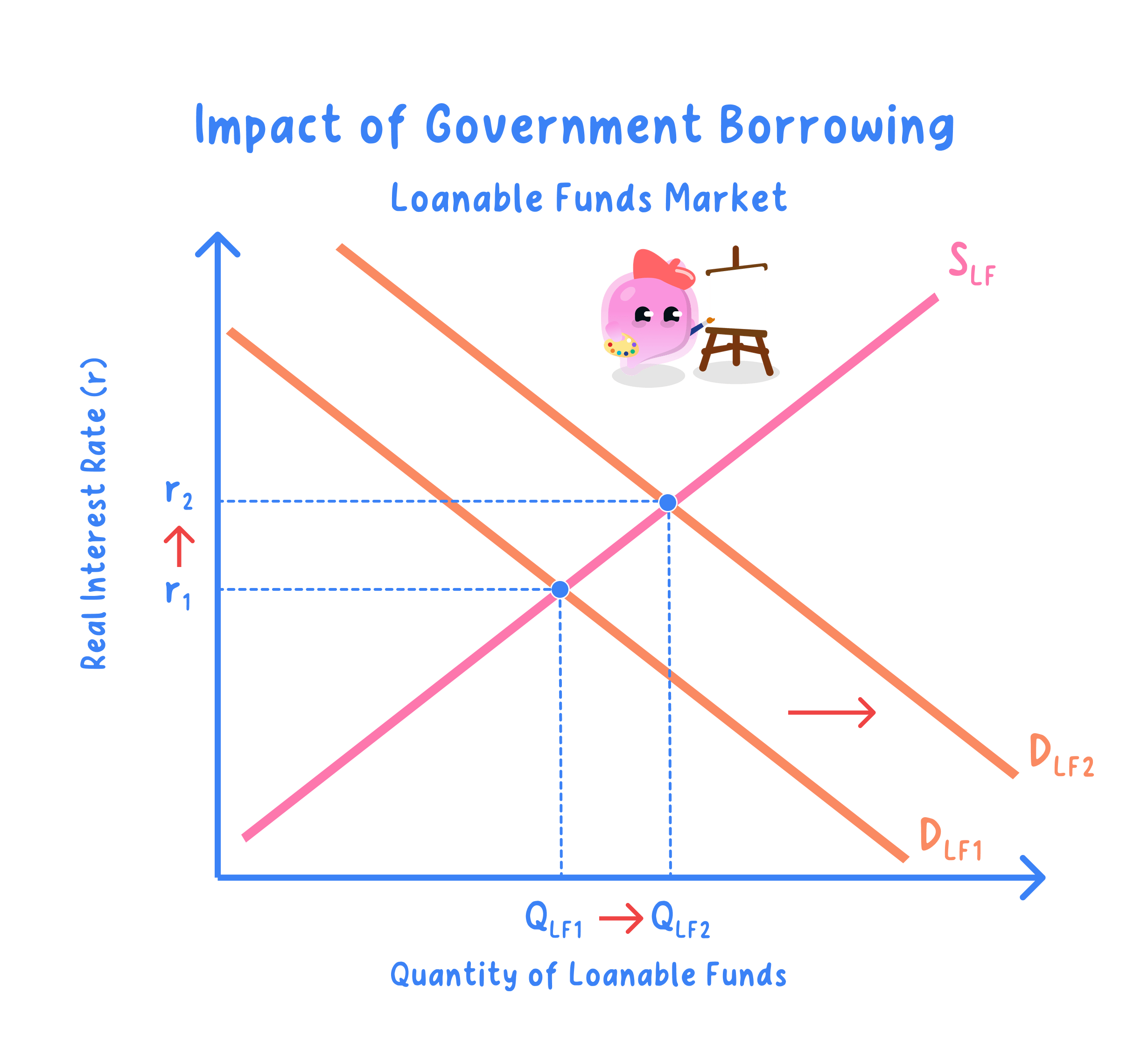
- Crowding out: extra borrowing can raise interest rates and displace private investment.
- The multiplier: if saving or import leakage is high, each £1 of spending circulates less and the effect is muted.
- Political constraints: governments may avoid unpopular tax rises or spending cuts, or act for electoral reasons.
- Fiscal policy is most effective in a deep recession with spare capacity, where the multiplier is large and crowding out is unlikely.
- Near full capacity the same policy mainly raises the price level, so it interacts with monetary policy and works best when the two pull in the same direction.
Worked example: the multiplier
Suppose the government raises spending by £10 billion and the marginal propensity to consume (MPC) is 0.6. The multiplier is 11−MPC=11−0.6=10.4=2.5\dfrac{1}{1 - \text{MPC}} = \dfrac{1}{1 - 0.6} = \dfrac{1}{0.4} = 2.51−MPC1=1−0.61=0.41=2.5.
Real national income eventually rises by £10bn×2.5=£25 billion\pounds 10\text{bn} \times 2.5 = \pounds 25\text{ billion}£10bn×2.5=£25 billion, provided there is spare capacity to meet the extra demand. If leakages into saving, tax and imports are larger so that the MPC is only 0.5, the multiplier falls to 222 and the same £10bn injection raises income by just £20 billion. The higher the leakages, the weaker the effect.
- Trace the full chain: a tax cut raises disposable income, which raises consumption and aggregate demand.
- Bring in the multiplier to show the size of the final effect.
- Evaluate using time lags, crowding out and the state of the economy, then reach a judgement rather than listing effects.
- Do not confuse fiscal policy (spending and taxation) with monetary policy (interest rates and the money supply).
- Do not assume fiscal policy always raises output; near full capacity it mainly raises the price level.
- Define expansionary and contractionary fiscal policy.
- How does fiscal policy affect aggregate demand?
- Explain how the multiplier changes the impact of government spending.
- Give two reasons fiscal policy may be ineffective.
- When is fiscal policy most effective, and why?
2.5.1b Public expenditure and taxation
Public Spending and Taxation: Types, Reasons and How Taxes Are Classified
Tax: A financial charge that governments collect from individuals and businesses.
Public expenditure divides into capital, current and transfer payments. Taxes are direct (on income and wealth) or indirect (on spending), and are progressive, proportional or regressive depending on how the average tax rate changes as income rises.
Types and Reasons for Public Expenditure
- Capital spending is investment in long-lived assets, such as new roads or hospitals.
- Current spending covers day-to-day running costs, such as public sector wages, state schools and defence.
- Transfer payments move income between groups, such as the State Pension and Universal Credit, and are not payment for output.
- Governments spend to provide public and merit goods, to redistribute income towards those in need, and to manage the level of aggregate demand.
- State schools and defence are current spending on services.
- The State Pension and Universal Credit are transfer payments, so they are not counted in national output.
Why Governments Tax, and Direct Versus Indirect Taxes
- Governments levy taxes to fund public spending, redistribute income, correct market failure and influence aggregate demand.
- Direct taxes are levied on income and wealth, such as income tax and National Insurance.
- Indirect taxes are levied on spending, such as VAT.
- A good tax is judged on principles such as equity (fairness), certainty, convenience and efficiency.
Progressive, Proportional and Regressive Taxes
- Progressive tax: the average rate rises as income rises, for example UK income tax.
- Proportional tax: the average rate stays constant as income rises.
- Regressive tax: the average rate falls as income rises, as with VAT, which takes a larger share of a low income.
- It is the average rate (tax paidincome×100\dfrac{\text{tax paid}}{\text{income}} \times 100incometax paid×100), not the marginal rate (the tax on the next £1 earned), that tells you whether a tax is progressive.
- The mix of taxes therefore shapes the distribution of income.
Worked Example: Average and Marginal Tax Rates
- Someone earning £30,000 who pays £6,000 in tax faces an average rate of £6,000£30,000×100=20%\dfrac{\pounds 6{,}000}{\pounds 30{,}000} \times 100 = 20\%£30,000£6,000×100=20%.
- If income rises to £40,000 and tax rises to £9,000, the extra £3,000 on the extra £10,000 is a marginal rate of £3,000£10,000×100=30%\dfrac{\pounds 3{,}000}{\pounds 10{,}000} \times 100 = 30\%£10,000£3,000×100=30%.
- The average rate rises from 20%20\%20% to £9,000£40,000×100=22.5%\dfrac{\pounds 9{,}000}{\pounds 40{,}000} \times 100 = 22.5\%£40,000£9,000×100=22.5%, so the tax is progressive.
- UK income tax is progressive for exactly this reason.
- A tax-free personal allowance (around £12,570) is followed by a 20 per cent basic rate, a 40 per cent higher rate and a 45 per cent additional rate.
- Even though each band has a fixed marginal rate, moving into higher bands pulls the average rate up, so higher earners pay a larger share of their income.
Weighing the Relative Merits of the Main UK Taxes
- Income tax is progressive and equitable and raises large, reliable revenue, but high marginal rates can weaken work incentives and encourage avoidance.
- VAT is broad-based, hard to evade and gives stable revenue, but it is regressive because it takes a larger share of a low income.
- Corporation tax raises substantial revenue, but can deter investment and weaken international competitiveness if set too high.
- Excise duties correct externalities and give stable revenue from inelastic demand, but are regressive and can encourage smuggling.
- Judge any tax against equity, efficiency, incentives and revenue stability; each UK tax trades some of these off against others.
- Classify spending as capital, current or a transfer, and give a clear reason for it.
- Classify a tax by what happens to the average rate as income rises.
- Distinguish direct taxes on income and wealth from indirect taxes on spending.
- Do not count transfer payments as part of national output; they redistribute income rather than pay for goods and services.
- Do not confuse a progressive tax with one that simply raises more revenue; what matters is that the average rate rises as income rises.
- Keep the average rate distinct from the marginal rate, which applies only to extra income.
- Name the three types of government spending.
- Give two reasons governments levy taxes.
- Distinguish direct from indirect taxes.
- Define progressive, proportional and regressive taxes in terms of the average rate.
- Why is VAT regressive?
- Give one merit and one drawback of income tax and of VAT.
2.5.1c Budget balances and the national debt
The Budget Balance Is a Yearly Flow; the National Debt Is the Accumulated Stock
Budget deficit: the amount by which government spending exceeds government revenue over a given period.
National debt: the total stock of government borrowing outstanding, accumulated from past budget deficits.
The budget balance is government spending minus tax revenue in a year. A deficit adds to the national debt, the total stock of past borrowing; a surplus reduces it.
The Budget Balance and Budget Positions
- Budget balance: the difference between government spending and tax revenue over a year.
- Budget deficit: spending exceeds revenue, so the government must borrow.
- Budget surplus: revenue exceeds spending, allowing debt to be repaid.
- A balanced budget is where the two are equal.
Deficit and Debt: A Flow and a Stock
- A fiscal (budget) deficit is a flow: the amount by which spending exceeds revenue in a single year.
- The national debt is a stock: the total accumulated past borrowing not yet repaid.
- Each year's deficit adds to the national debt, while a surplus reduces it.
- Think of a bath: the deficit is the flow from the tap, and the debt is the water in the bath.
- So the debt can keep rising even when the deficit is falling, because a smaller deficit still adds to the stock, just more slowly.
Worked example: how a deficit feeds the debt
Suppose the national debt starts the year at £2,500 billion and the government runs a budget deficit of £100 billion. The debt rises to £2,500bn+£100bn=£2,600 billion\pounds 2{,}500\text{bn} + \pounds 100\text{bn} = \pounds 2{,}600\text{ billion}£2,500bn+£100bn=£2,600 billion.
The next year the deficit is cut to £80 billion. The debt still rises, to £2,600bn+£80bn=£2,680 billion\pounds 2{,}600\text{bn} + \pounds 80\text{bn} = \pounds 2{,}680\text{ billion}£2,600bn+£80bn=£2,680 billion, because a smaller deficit is still fresh borrowing added to the stock. Only an actual surplus would reduce the debt.
- The debt is usually judged as a share of GDP, not in cash terms, so a growing economy can carry a rising debt if GDP grows faster.
Cyclical and Structural Deficits and Surpluses
- A cyclical deficit arises because output is below trend, with lower tax revenue and higher benefit spending; it fades as the economy recovers.
- A structural deficit remains even at the trend level of output and needs policy action to remove.
- The balance moves automatically over the cycle, improving in a boom and worsening in a downturn, so sustainability depends mainly on the structural part.
Consequences and the Significance of the National Debt
- A deficit can support aggregate demand in a recession, while a surplus withdraws demand; persistent deficits add to the debt.
- A large debt must be serviced with interest, which has an opportunity cost in lost spending on schools or hospitals and raises questions of fairness between generations.
- A very high debt can risk a credit downgrade and higher borrowing costs.
- A rising debt is not automatically harmful, though: borrowing to fund investment can raise future output, so the cost of borrowing must be weighed against the return on what it finances and the size of the debt relative to GDP.
- Define the deficit as a yearly flow and the debt as the accumulated stock, and never mix the two up.
- Split a deficit into cyclical and structural parts, and base the policy response on the structural part.
- Judge the debt relative to GDP, weighing the cost of borrowing against the return on what it funds.
- Do not use deficit and debt as if they mean the same thing; the deficit is a flow and the debt is a stock.
- Do not say that cutting the deficit reduces the debt; a smaller deficit still adds to the debt, just more slowly.
- Do not assume any rise in the national debt is automatically harmful.
- What is a fiscal deficit, and what is the national debt?
- How are the deficit and the debt related?
- Distinguish a cyclical from a structural deficit.
- Can the debt rise while the deficit falls? Explain.
- Why is the debt usually measured as a share of GDP?
2.5.1d The Office for Budget Responsibility
The OBR Is an Independent Forecaster and Scrutineer, Not a Policymaker
Office for Budget Responsibility: the independent public body that produces official forecasts of the UK economy and public finances and assesses the government's performance against its fiscal targets.
The Office for Budget Responsibility (OBR) is the UK's independent fiscal watchdog. It produces the official economic and fiscal forecasts and judges performance against the government's fiscal rules, but it does not set fiscal policy.
- The OBR was set up in 2010 to bring independent, transparent forecasting to the Budget process, ending the previous practice in which the Treasury produced its own forecasts and could be tempted to present them favourably.
What the OBR Does
- Independent forecasts: it produces the official economic and fiscal forecasts, published in its Economic and Fiscal Outlook at least twice a year alongside the Budget.
- Scrutiny of costings: it scrutinises the costing of the government's tax and spending measures.
- Sustainability: it assesses the long-run sustainability of the public finances and reports on the outlook for the national debt.
- It judges whether the government is on track to meet its fiscal rules.
Why Independence Matters
- An independent body improves transparency and reduces the temptation to publish over-optimistic forecasts.
- This raises the credibility of fiscal policy in the eyes of investors who lend to the government.
- Even so, forecasting is inherently uncertain, so OBR projections are frequently revised as new data arrive and should not be treated as guaranteed outcomes.
In September 2022 the government's mini-Budget announced large unfunded tax cuts without an accompanying OBR forecast. The absence of independent scrutiny contributed to a sharp fall in the pound and a spike in government borrowing costs, showing how much financial markets value the OBR's independent judgement.
- Describe the OBR as an independent forecaster and scrutineer.
- Link its role to the credibility of the public finances.
- Be clear that it does not set fiscal policy; the government does.
- Do not treat the OBR as setting fiscal policy; it forecasts and scrutinises, while the government sets policy.
- What is the OBR?
- Name two things it does.
- Why does independence improve credibility?
- Does the OBR set fiscal policy?
