

What you'll learn
- How production changes as a firm adds more workers in the short run.
- How to calculate total, average and marginal costs and revenues.
- Why long-run average cost can fall, flatten, then rise as firms grow.
- How economists decide whether a firm is earning normal or abnormal profit.
The big picture: firms, output and profit
A firm is an organisation that combines factors of production — land, labour, capital and enterprise — to produce output, meaning goods or services.
Firms make decisions about how much to produce by comparing:
- costs: what they must give up to produce output
- revenues: money received from selling output
- profits: the surplus left after costs are deducted from revenue
A key idea in this topic is marginal thinking. “Marginal” means the extra amount created by one more unit of activity — for example, one more worker, one more product, or one more unit sold.
Short run, long run and diminishing returns
Short run and long run
- The short run is a period of time in which at least one factor of production is fixed, such as factory space or machinery.
- The long run is a period of time in which all factors of production can be changed.
In the short run, a firm may be able to hire more workers quickly, but it may not be able to expand its factory or buy new machinery immediately. That matters because extra workers eventually have less fixed capital to work with.
Law of diminishing returns
The law of diminishing returns states that, in the short run, adding more units of a variable factor to a fixed factor will eventually cause marginal product to fall.
This does not mean output immediately falls. Total output may still rise, but it rises more slowly because each extra worker adds less extra output than the previous worker.
The diagram shows total product, average product and marginal product in the short run.
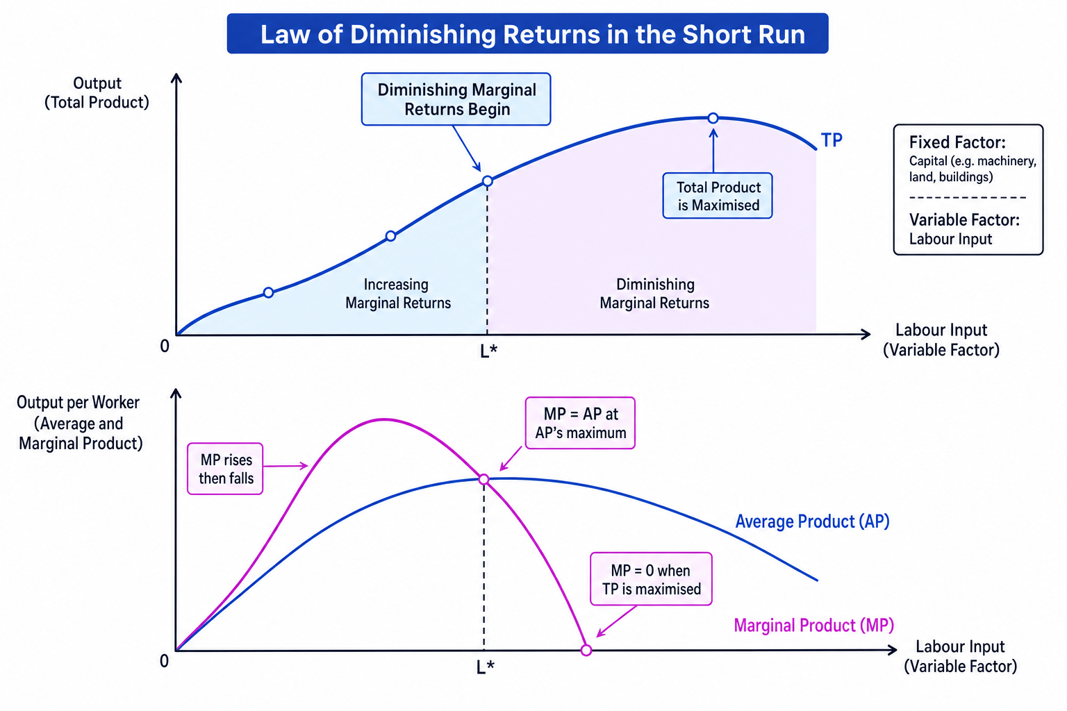
Total, average and marginal product
Product measures
- Total product (TP) is the total output produced.
- Average product (AP) is output per unit of the variable factor.
- Marginal product (MP) is the extra output produced by employing one more unit of the variable factor.
where LLL is labour.
Calculating product and identifying diminishing returns
A café has one fixed coffee machine. As it hires workers from 1 to 5, total output per hour is 20, 50, 75, 92 and 100 coffees.
- Calculate marginal product by finding the extra coffees from each extra worker: 20, 30, 25, 17 and 8 coffees.
- Calculate average product: with 2 workers, AP is 50 divided by 2 = 25 coffees per worker; with 4 workers, AP is 92 divided by 4 = 23 coffees per worker.
- Identify where diminishing marginal returns begin: MP rises from 20 to 30, then falls to 25 when the third worker is added, so diminishing marginal returns begin after 2 workers.
- Link this to costs: if each worker costs £100 per hour, the second worker adds 30 coffees, costing £3.33 per extra coffee, while the fifth adds only 8 coffees, costing £12.50 per extra coffee.
Product and cost are linked
When marginal product falls, marginal cost tends to rise, because the firm is paying for extra labour but receiving fewer extra units of output.
Short-run costs
Fixed and variable costs
- Fixed costs do not change with output in the short run, such as rent, insurance or loan repayments.
- Variable costs change as output changes, such as raw materials, packaging or hourly wages.
Total, average and marginal cost are central to this topic.
TC=TFC+TVCAFC=TFCQAVC=TVCQATC=TCQMC=ΔTCΔQ\begin{aligned} TC &= TFC + TVC \\ AFC &= \frac{TFC}{Q} \\ AVC &= \frac{TVC}{Q} \\ ATC &= \frac{TC}{Q} \\ MC &= \frac{\Delta TC}{\Delta Q} \end{aligned}TCAFCAVCATCMC=TFC+TVC=QTFC=QTVC=QTC=ΔQΔTCwhere QQQ is output.
- Total cost (TC) is all costs of production.
- Total fixed cost (TFC) is all fixed costs.
- Total variable cost (TVC) is all variable costs.
- Average fixed cost (AFC) is fixed cost per unit.
- Average variable cost (AVC) is variable cost per unit.
- Average total cost (ATC) is total cost per unit.
- Marginal cost (MC) is the extra cost of producing one more unit.
The short-run cost curves and long-run average cost curve are shown below.
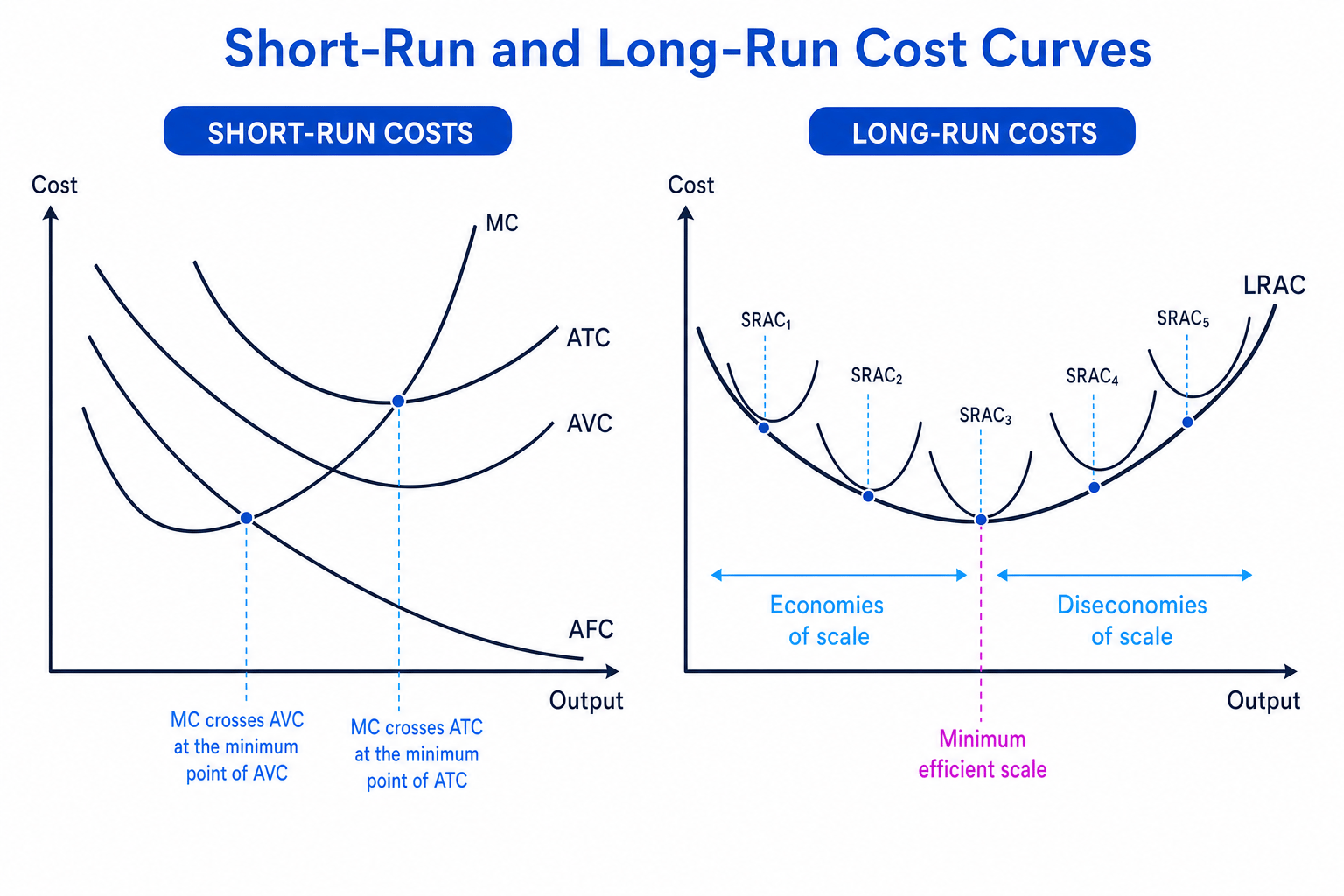
Averages and marginals
If MC is below an average cost curve, it pulls the average down. If MC is above it, it pulls the average up. Therefore MC cuts AVC and ATC at their minimum points.
Calculating total, average and marginal cost
A firm has fixed costs of £500. At 100 units, variable costs are £800. At 120 units, variable costs are £1,040.
- Calculate total cost at 100 units: £500 + £800 = £1,300.
- Calculate average total cost at 100 units: £1,300 divided by 100 = £13 per unit.
- Calculate total cost at 120 units: £500 + £1,040 = £1,540.
- Calculate marginal cost over this output range: total cost rises by £240 and output rises by 20 units, so MC = £12 per extra unit.
Fixed cost does not mean average fixed cost is fixed
Total fixed cost stays the same in the short run, but average fixed cost falls as output rises because the same fixed cost is spread over more units.
Revenue
Revenue measures
- Total revenue (TR) is the total money received from sales.
- Average revenue (AR) is revenue per unit sold.
- Marginal revenue (MR) is the extra revenue from selling one more unit.
If a firm sells all units at the same price, AR is the same as price. In a perfectly competitive market, firms are price takers, so AR and MR are constant. In less competitive markets, a firm may have to cut price to sell more, so MR lies below AR.
Calculating total, average and marginal revenue
A firm sells 100 units at £10 each. To sell 110 units, it cuts price to £9.50.
- Calculate initial total revenue: £10 times 100 = £1,000.
- Calculate new total revenue: £9.50 times 110 = £1,045.
- Calculate marginal revenue over the extra 10 units: revenue rises by £45, so MR = £4.50 per extra unit.
- Compare MR with price: MR is below £9.50 because the lower price applies to all units sold, not just the extra units.
Economies and diseconomies of scale
In the long run, all factors can vary, so the firm can choose its scale of production. The long-run average cost (LRAC) curve is derived from the lowest possible short-run average cost at each output level. This is why it is often called an “envelope” of short-run average cost curves.
Economies and diseconomies of scale
- Economies of scale occur when LRAC falls as output rises.
- Diseconomies of scale occur when LRAC rises as output rises.
- Minimum efficient scale is the lowest level of output where LRAC is minimised.
Internal economies and diseconomies
Internal economies of scale arise from growth within the firm. Examples include:
- purchasing economies from bulk buying
- technical economies from more efficient machinery
- managerial economies from specialist managers
- financial economies from easier access to cheaper borrowing
Internal diseconomies of scale arise when the firm becomes too large to manage efficiently. Communication worsens, decision-making slows, and workers may feel less motivated.
External economies and diseconomies
External economies of scale arise from growth of the whole industry or area, not just one firm. For example, a cluster of tech firms may attract skilled workers and specialist suppliers.
External diseconomies of scale also come from industry-wide growth, such as congestion, higher local wages, rising rents or pressure on infrastructure.
Interpreting long-run average cost
A manufacturer’s LRAC is £8 at 1,000 units, £5 at 5,000 units, £5 at 10,000 units and £6.50 at 16,000 units.
- Compare 1,000 with 5,000 units: LRAC falls from £8 to £5, so the firm experiences economies of scale.
- Compare 5,000 with 10,000 units: LRAC stays at £5, so the firm has reached the lowest-cost range; minimum efficient scale begins at 5,000 units.
- Compare 10,000 with 16,000 units: LRAC rises from £5 to £6.50, so diseconomies of scale are occurring.
Profit: accounting, economic, normal and abnormal
Businesses and economists use profit differently.
Accounting profit and economic profit
- Accounting profit is total revenue minus explicit costs, such as wages, rent and raw materials.
- Economic profit is total revenue minus both explicit costs and implicit opportunity costs.
An implicit cost is the value of the next best alternative given up. For example, if an entrepreneur could earn £35,000 elsewhere, that forgone salary is an implicit cost of running the business.
Normal and abnormal profit
- Normal profit is the minimum return needed to keep enterprise in its current use. It is included as part of economic cost.
- Abnormal profit is profit above normal profit. It exists when economic profit is positive.
Calculating accounting and economic profit
A small business earns total revenue of £200,000. Explicit costs are £150,000. The owner gives up a £35,000 salary elsewhere and could have earned £10,000 by investing their capital differently.
- Calculate accounting profit: £200,000 - £150,000 = £50,000.
- Add opportunity costs to find economic cost: £150,000 + £35,000 + £10,000 = £195,000.
- Calculate economic profit: £200,000 - £195,000 = £5,000, so the firm earns £5,000 abnormal profit.
- Interpret the result: if economic profit were zero, the firm would still be earning normal profit.
Profit maximisation: using MR and MC
A firm maximises profit where marginal revenue equals marginal cost, as long as MC is rising at that output.
If MR is greater than MC, producing more adds more to revenue than to cost, so profit rises. If MC is greater than MR, producing more adds more to cost than to revenue, so profit falls.
The diagram shows profit maximisation for a firm with downward-sloping demand.
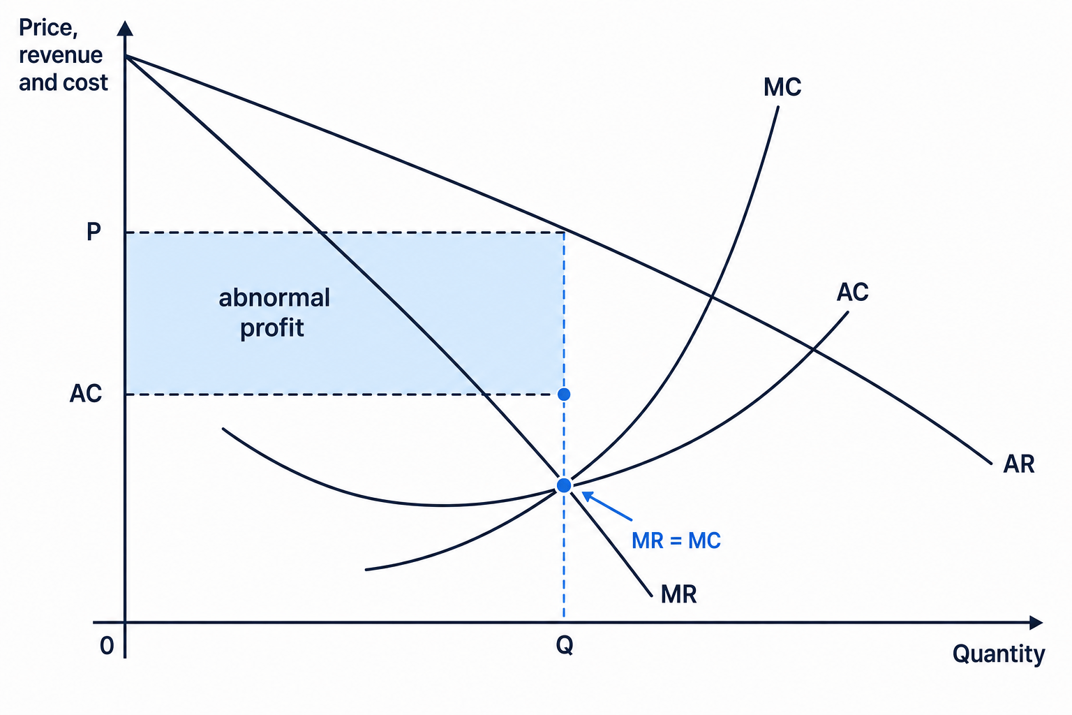
At the profit-maximising output:
- if AR is above AC, the firm earns abnormal profit
- if AR equals AC, the firm earns normal profit
- if AR is below AC, the firm makes an economic loss
Finding profit-maximising output and profit
A firm finds that MR = MC at 110 units. At this output, AR is £14 and AC is £11.
- Choose 110 units because this is where the extra revenue from the last unit equals the extra cost of producing it.
- Find profit per unit: AR - AC = £14 - £11 = £3.
- Calculate total profit: £3 times 110 units = £330 abnormal profit.
MR equals MC is not enough on its own
The profit-maximising rule requires MC to cut MR from below. If MC is falling at the intersection, that point may not be maximum profit.
In the exam
- Define the key term first, then use the correct formula with units: £, units, or £ per unit.
- For diagrams, label axes clearly and show the relevant output, price, cost or profit area.
- When evaluating, separate short-run effects from long-run effects, especially for diminishing returns and economies of scale.
Check yourself
- Why does marginal cost rise when marginal product falls?
- How is economic profit different from accounting profit?
- What does it mean if a firm produces where MR = MC but AR = AC?
