What you'll learn

• How aggregate demand (AD) and aggregate supply (AS) interact in the macroeconomy.
• How to read and draw AD/AS diagrams with real GDP, employment and the price level.
• How short-run shocks become long-run outcomes using SRAS and LRAS.
• How to build strong AO3/AO4 analysis from AD/AS diagrams.

The basic macroeconomic picture

AD/AS analysis is the macroeconomic equivalent of demand and supply in a market, but the “market” is the whole economy.

The vertical axis is the price level, meaning the average level of prices across the economy, often measured using an index such as CPI. The horizontal axis is real GDP, meaning the value of national output adjusted for inflation.

As real GDP rises, firms usually need more workers, so employment tends to rise and unemployment tends to fall. This is why AD/AS diagrams can explain output, employment and prices together.

AD is made up of four components:

$$AD=C+I+G+(X-M)$$

Where C is consumption, I is investment, G is government spending, X is exports and M is imports.

Why AD slopes downwards

The AD curve slopes down from left to right because a higher price level tends to reduce total spending:

• Real balance effect: inflation reduces the real value of people’s savings, so they may spend less.
• Interest rate effect: higher prices can increase demand for money, pushing interest rates up and reducing consumption and investment.
• International competitiveness effect: if UK prices rise relative to other countries, exports may fall and imports may rise.

Aggregate supply: what the economy can produce

Economists usually separate AS into the short run and the long run.

Short-run aggregate supply

Short-run aggregate supply (SRAS) shows planned output when some costs, especially wages, are fixed or slow to change.

SRAS slopes upward because higher prices can make production more profitable in the short run. If firms receive higher prices while wages and other input costs have not fully adjusted, they have an incentive to expand output.

SRAS shifts when production costs change. For example:

• Higher oil, gas or wage costs shift SRAS left.
• Better productivity or lower business taxes can shift SRAS right.
• A weaker pound can shift SRAS left if imported raw materials become more expensive.

The UK’s 2021–23 cost-of-living squeeze is a useful context: global supply-chain disruption and higher energy prices raised firms’ costs, contributing to cost-push inflation.

Long-run aggregate supply

In the classical or neoclassical model, LRAS is vertical at full-employment output, often labelled $Y_{FE}$. This means the economy has a maximum sustainable level of output determined by the quantity and quality of land, labour, capital and enterprise.

Full employment does not mean zero unemployment. It means the economy is producing at its sustainable capacity, with no cyclical unemployment, though frictional and structural unemployment may still exist.

Long-run equilibrium in AD/AS

The economy is in macroeconomic equilibrium where AD equals AS. In a classical long-run diagram, long-run equilibrium occurs where AD, SRAS and LRAS all intersect.

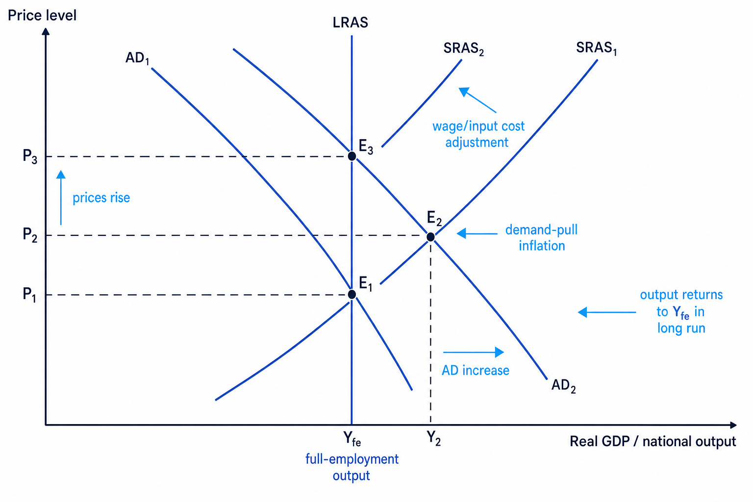
At $E_1$, the economy is at full-employment output $Y_{FE}$ and price level $P_1$.

If AD increases, the economy moves to $E_2$ in the short run. Real GDP rises above sustainable capacity, so employment rises and unemployment falls below its natural level. But this creates pressure on wages and input prices. Eventually SRAS shifts left, moving the economy to $E_3$: output returns to $Y_{FE}$, but the price level is higher.

What shifts AD, SRAS and LRAS?

AD shifts

AD shifts right when total spending rises. This could be caused by:

• Lower interest rates increasing borrowing and spending.
• Tax cuts increasing disposable income.
• Higher government spending.
• A depreciation of the pound making UK exports cheaper and imports more expensive.
• Improved business or consumer confidence.

AD shifts left when these factors reverse. For example, Bank of England interest-rate rises during 2021–23 were intended to reduce inflation partly by weakening borrowing, consumption and investment.

SRAS shifts

SRAS changes when firms’ short-run costs change. For example, Brexit-related trade frictions, higher import prices or energy shocks can shift SRAS left. Improved logistics, lower energy costs or better labour productivity can shift SRAS right.

LRAS shifts

LRAS changes when the economy’s productive potential changes. LRAS shifts right if the economy can sustainably produce more. Causes include:

• Higher investment in capital equipment.
• Better education and training.
• Improved infrastructure.
• Technological progress.
• Higher labour-force participation.
• More efficient institutions and regulation.

For example, investment in transport infrastructure in an emerging economy such as India could raise productivity and shift LRAS right over time.

Keynesian AD/AS: spare capacity matters

The Keynesian model suggests the effect of AD depends on how much spare capacity exists in the economy.

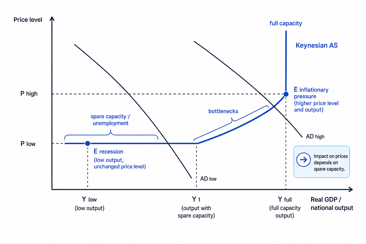
When there is lots of spare capacity, firms can increase output without much pressure on prices. AD increases mainly raise real GDP and employment.

Near full capacity, extra AD is more likely to cause inflation because firms compete for scarce workers, materials and factory space.

Output gaps and employment

An output gap is the difference between actual real GDP and potential output.

A negative output gap occurs when actual GDP is below potential GDP. This suggests spare capacity and cyclical unemployment.

A positive output gap occurs when actual GDP is above potential GDP. This suggests overheating and inflationary pressure.

Employment links directly to this analysis. When output rises because AD increases, firms tend to hire more labour. But if output rises beyond sustainable capacity, the long-run adjustment may push employment back towards its sustainable level as costs rise and output falls back to $Y_{FE}$.

Building strong analysis chains

A good AD/AS paragraph normally follows this order:

1. Identify the shock or policy.
2. State which curve shifts and why.
3. Explain the new equilibrium price level and real GDP.
4. Link real GDP to employment.
5. Evaluate using spare capacity, time period, size of shift and whether SRAS or LRAS also changes.

For example, a cut in income tax may increase disposable income, shifting AD right. In the short run this may increase real GDP and employment, but if the economy is close to full capacity it may mainly cause inflation. In the long run, unless productive capacity improves, output returns towards $Y_{FE}$.