

What you'll learn
- How to distinguish random errors from systematic errors.
- What physicists mean by precision, accuracy, repeatability, reproducibility and resolution.
- How to calculate absolute, fractional and percentage uncertainties.
- How to use error bars to estimate uncertainty in a graph’s gradient and intercept.
Measurements are always estimates
In physics, a measurement is never perfectly exact. Instruments have limited resolution, humans make judgement calls, and experimental conditions vary. The aim is not to get a “perfect” answer, but to estimate how trustworthy your result is.
Error and uncertainty
- Error is the difference between a measured value and the true value. The true value is the value you would get with a perfect measurement, which is usually not known exactly.
- Uncertainty is the estimated range within which the true value is expected to lie. A result written as x±Δxx \pm \Delta xx±Δx means the best estimate is xxx, with absolute uncertainty Δx\Delta xΔx.
The big idea
Uncertainty is not a sign that the experiment has “gone wrong”. It is a measured, honest statement of the limits of your result.
Random and systematic errors
The two main types of error behave very differently. This target picture is a useful way to remember the difference: random error causes spread, while systematic error causes a shift.
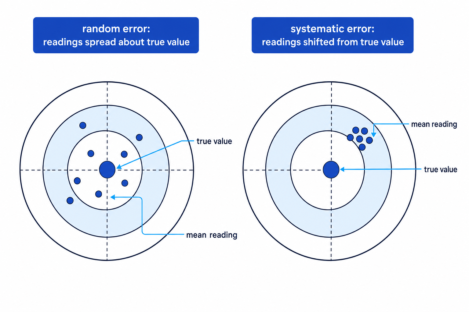
Random and systematic errors
- A random error causes repeated readings to vary unpredictably around a mean value.
- A systematic error shifts all readings in the same direction, usually because of a fault in the method or instrument.
Random errors can often be reduced by taking repeat readings and calculating a mean. Systematic errors must be removed or corrected, for example by zeroing an instrument, calibrating it, or changing the method.
Identifying error types
A student uses an ammeter. It reads 0.03 A when no current is flowing. During the experiment, repeated readings for a steady current vary between 0.41 A and 0.45 A.
- The 0.03 A reading when there is no current is a zero error, so every reading is shifted upwards. This is a systematic error.
- The variation between 0.41 A and 0.45 A for the same current is a spread in repeated readings. This is a random error.
- To improve the experiment, the student should zero or correct the ammeter to deal with the systematic error, and take repeated readings and a mean to reduce the effect of random error.
Describing the quality of measurements
These words are easy to mix up, but examiners use them very specifically.
Measurement quality words
- Accuracy means closeness to the true value.
- Precision means repeated readings are close to each other, or that a value is quoted to a fine level of detail.
- Repeatability means the same person, using the same equipment and method, gets similar results when repeating the experiment.
- Reproducibility means different people, equipment, methods or laboratories get similar results.
- Resolution is the smallest change an instrument can detect or display.
A digital thermometer that reads to 0.1 K has a resolution of 0.1 K. A ruler marked every 1 mm has a resolution of 1 mm, which is 0.001 m.
Precision is not accuracy
A set of readings can be very precise but still inaccurate. For example, a miscalibrated balance may give very consistent mass readings, but all of them may be too high.
For a single reading, uncertainty is often linked to resolution. In many school practicals, an analogue scale is taken as about half the smallest division, while a digital display is often taken as one unit in the last displayed digit. If the question gives an uncertainty, use the given value.
Absolute, fractional and percentage uncertainty
An absolute uncertainty has the same unit as the quantity. For example, L=0.842±0.001 mL = 0.842 \pm 0.001\ \text{m}L=0.842±0.001 m has absolute uncertainty 0.001 m.
A fractional uncertainty compares the absolute uncertainty with the measured value:
fractional uncertainty=Δxx\text{fractional uncertainty} = \frac{\Delta x}{x}fractional uncertainty=xΔxA percentage uncertainty is the fractional uncertainty written as a percentage:
percentage uncertainty=Δxx×100%\text{percentage uncertainty} = \frac{\Delta x}{x} \times 100\%percentage uncertainty=xΔx×100%If repeated readings are taken, a simple A-Level method is to estimate the absolute uncertainty using half the range:
Δx=xmax−xmin2\Delta x = \frac{x_{\text{max}} - x_{\text{min}}}{2}Δx=2xmax−xminEstimating uncertainty from repeated readings
A student measures a time four times: 1.22 s, 1.25 s, 1.24 s and 1.23 s.
-
Calculate the mean time:
T=1.22+1.25+1.24+1.234=1.235 sT = \frac{1.22 + 1.25 + 1.24 + 1.23}{4} = 1.235\ \text{s}T=41.22+1.25+1.24+1.23=1.235 s -
Estimate the absolute uncertainty using half the range:
ΔT=1.25−1.222=0.015 s\Delta T = \frac{1.25 - 1.22}{2} = 0.015\ \text{s}ΔT=21.25−1.22=0.015 s -
Calculate the percentage uncertainty:
0.0151.235×100%=1.2%\frac{0.015}{1.235} \times 100\% = 1.2\%1.2350.015×100%=1.2% -
Quote the result sensibly as T=1.24±0.02 sT = 1.24 \pm 0.02\ \text{s}T=1.24±0.02 s.
Significant figures and uncertainty
Usually quote the uncertainty to one significant figure, or sometimes two if the first digit is 1 or 2. Then round the measured value to the same decimal place as the uncertainty.
Combining uncertainties
When a final answer is calculated from measurements, the uncertainties must be combined using the correct rule.
For addition or subtraction, add absolute uncertainties:
Q=a+b or a−b⇒ΔQ=Δa+ΔbQ = a + b \text{ or } a - b \Rightarrow \Delta Q = \Delta a + \Delta bQ=a+b or a−b⇒ΔQ=Δa+ΔbFor multiplication or division, add fractional or percentage uncertainties:
Q=ab or ab⇒ΔQQ=Δaa+ΔbbQ = ab \text{ or } \frac{a}{b} \Rightarrow \frac{\Delta Q}{Q} = \frac{\Delta a}{a} + \frac{\Delta b}{b}Q=ab or ba⇒QΔQ=aΔa+bΔbFor powers, multiply the fractional or percentage uncertainty by the power:
Q=an⇒ΔQQ=∣n∣ΔaaQ = a^n \Rightarrow \frac{\Delta Q}{Q} = |n|\frac{\Delta a}{a}Q=an⇒QΔQ=∣n∣aΔaFor example, if A=πr2A = \pi r^2A=πr2, the percentage uncertainty in AAA due to rrr is twice the percentage uncertainty in rrr. The constant π\piπ does not add uncertainty.
Combining uncertainties in speed
A trolley moves from x1=0.124±0.001 mx_1 = 0.124 \pm 0.001\ \text{m}x1=0.124±0.001 m to x2=0.856±0.001 mx_2 = 0.856 \pm 0.001\ \text{m}x2=0.856±0.001 m in t=1.42±0.01 st = 1.42 \pm 0.01\ \text{s}t=1.42±0.01 s.
-
Calculate the displacement and add absolute uncertainties because the positions are subtracted:
s=0.856−0.124=0.732 ms = 0.856 - 0.124 = 0.732\ \text{m}s=0.856−0.124=0.732 m Δs=0.001+0.001=0.002 m\Delta s = 0.001 + 0.001 = 0.002\ \text{m}Δs=0.001+0.001=0.002 m -
Convert the displacement and time uncertainties to percentages:
0.0020.732×100%=0.273%\frac{0.002}{0.732} \times 100\% = 0.273\%0.7320.002×100%=0.273% 0.011.42×100%=0.704%\frac{0.01}{1.42} \times 100\% = 0.704\%1.420.01×100%=0.704% -
Since v=stv = \frac{s}{t}v=ts, add the percentage uncertainties:
0.273%+0.704%=0.977%0.273\% + 0.704\% = 0.977\%0.273%+0.704%=0.977% -
Calculate the speed and its absolute uncertainty:
v=0.7321.42=0.515 m s−1v = \frac{0.732}{1.42} = 0.515\ \text{m s}^{-1}v=1.420.732=0.515 m s−1 Δv=0.00977×0.515=0.005 m s−1\Delta v = 0.00977 \times 0.515 = 0.005\ \text{m s}^{-1}Δv=0.00977×0.515=0.005 m s−1 -
Quote the final result as v=0.515±0.005 m s−1v = 0.515 \pm 0.005\ \text{m s}^{-1}v=0.515±0.005 m s−1.
Subtracting values does not subtract uncertainties
If you calculate a difference such as x2−x1x_2 - x_1x2−x1, the absolute uncertainties still add. Uncertainties represent possible spread, not signed numbers.
Error bars on graphs
An error bar shows the uncertainty range for a plotted data point. A vertical error bar shows uncertainty in the y-value; a horizontal error bar shows uncertainty in the x-value. Some points may have error bars and others may not, depending on what uncertainties are known.
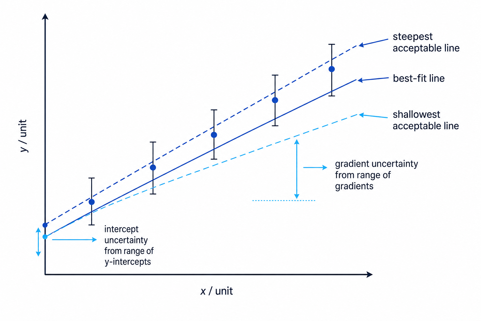
For a straight-line graph, draw a best-fit line, then draw the steepest and shallowest acceptable lines that still fit the error bars reasonably. These give the uncertainty in the gradient and intercept.
The gradient is found from:
gradient=ΔyΔx\text{gradient} = \frac{\Delta y}{\Delta x}gradient=ΔxΔyThe y-intercept is the value of yyy where the line crosses the y-axis.
If the maximum and minimum acceptable gradients are GmaxG_{\text{max}}Gmax and GminG_{\text{min}}Gmin, then:
ΔG=Gmax−Gmin2\Delta G = \frac{G_{\text{max}} - G_{\text{min}}}{2}ΔG=2Gmax−GminSimilarly, for the intercept ccc:
Δc=cmax−cmin2\Delta c = \frac{c_{\text{max}} - c_{\text{min}}}{2}Δc=2cmax−cminFinding uncertainty in gradient and intercept
For a graph of force against extension, the best-fit gradient is 24.0 N m−124.0\ \text{N m}^{-1}24.0 N m−1. The steepest acceptable gradient is 25.6 N m−125.6\ \text{N m}^{-1}25.6 N m−1 and the shallowest acceptable gradient is 22.8 N m−122.8\ \text{N m}^{-1}22.8 N m−1. The possible intercepts range from 0.11 N to 0.26 N, with a best intercept of 0.18 N.
-
Calculate the gradient uncertainty from half the range:
ΔG=25.6−22.82=1.4 N m−1\Delta G = \frac{25.6 - 22.8}{2} = 1.4\ \text{N m}^{-1}ΔG=225.6−22.8=1.4 N m−1 -
Quote the gradient with its uncertainty:
G=24.0±1.4 N m−1G = 24.0 \pm 1.4\ \text{N m}^{-1}G=24.0±1.4 N m−1 -
Calculate the intercept uncertainty:
Δc=0.26−0.112=0.075 N\Delta c = \frac{0.26 - 0.11}{2} = 0.075\ \text{N}Δc=20.26−0.11=0.075 N -
Round sensibly and quote the intercept:
c=0.18±0.08 Nc = 0.18 \pm 0.08\ \text{N}c=0.18±0.08 N
In the exam
- Always decide whether uncertainties should be combined as absolute uncertainties or percentage uncertainties before calculating.
- For graphs, use large gradient triangles and include units for both gradient and intercept.
- If asked how to improve an experiment, say whether your suggestion reduces random error, removes systematic error, or improves resolution.
Check yourself
- Why does taking repeats reduce the effect of random error but not systematic error?
- When do you add absolute uncertainties, and when do you add percentage uncertainties?
- How would you use error bars to find the uncertainty in a graph’s gradient?
