The multiplier and the accelerator

What you'll learn

How injections, leakages and marginal propensities determine the national income multiplier.
How to calculate average and marginal propensities, plus the size of the multiplier.
Why the accelerator can make investment and the economic cycle more volatile.
How to explain and evaluate output gaps using AD-AS and PPC diagrams.

Start point: AD, income and the circular flow

Definition

Aggregate demand

Aggregate demand (AD) is total planned spending in an economy at a given price level. In an open economy, $A D = C + I + G + (X - M)$ , where consumption is $C$ , investment is $I$ , government spending is $G$ , exports are $X$ and imports are $M$ .

National income is the value of output produced in an economy over a period of time. In macroeconomics, output, income and expenditure are linked: when firms produce more output, households receive more income, which can then become more spending.

An injection is spending entering the circular flow: investment, government spending or exports. A withdrawal or leakage is income not passed on as domestic consumption: saving, taxation or imports.

So, an initial rise in government spending, exports or investment can cause a bigger final rise in national income — but only if enough of the extra income is re-spent rather than leaked away.

Average and marginal propensities

Definition

Average and marginal propensities

An average propensity measures a proportion of total income. A marginal propensity measures a proportion of an extra change in income. If $Y$ is income, $C$ is consumption, $S$ is saving and $W$ is total withdrawals:

APC=CY,MPC=ΔCΔYAPS=SY,MPS=ΔSΔYAPW=WY,MPW=ΔWΔY\begin{aligned} \text{APC} &= \frac{C}{Y}, \quad \text{MPC} = \frac{\Delta C}{\Delta Y}\\ \text{APS} &= \frac{S}{Y}, \quad \text{MPS} = \frac{\Delta S}{\Delta Y}\\ \text{APW} &= \frac{W}{Y}, \quad \text{MPW} = \frac{\Delta W}{\Delta Y} \end{aligned}

The marginal propensity to withdraw (MPW) includes all marginal leakages:

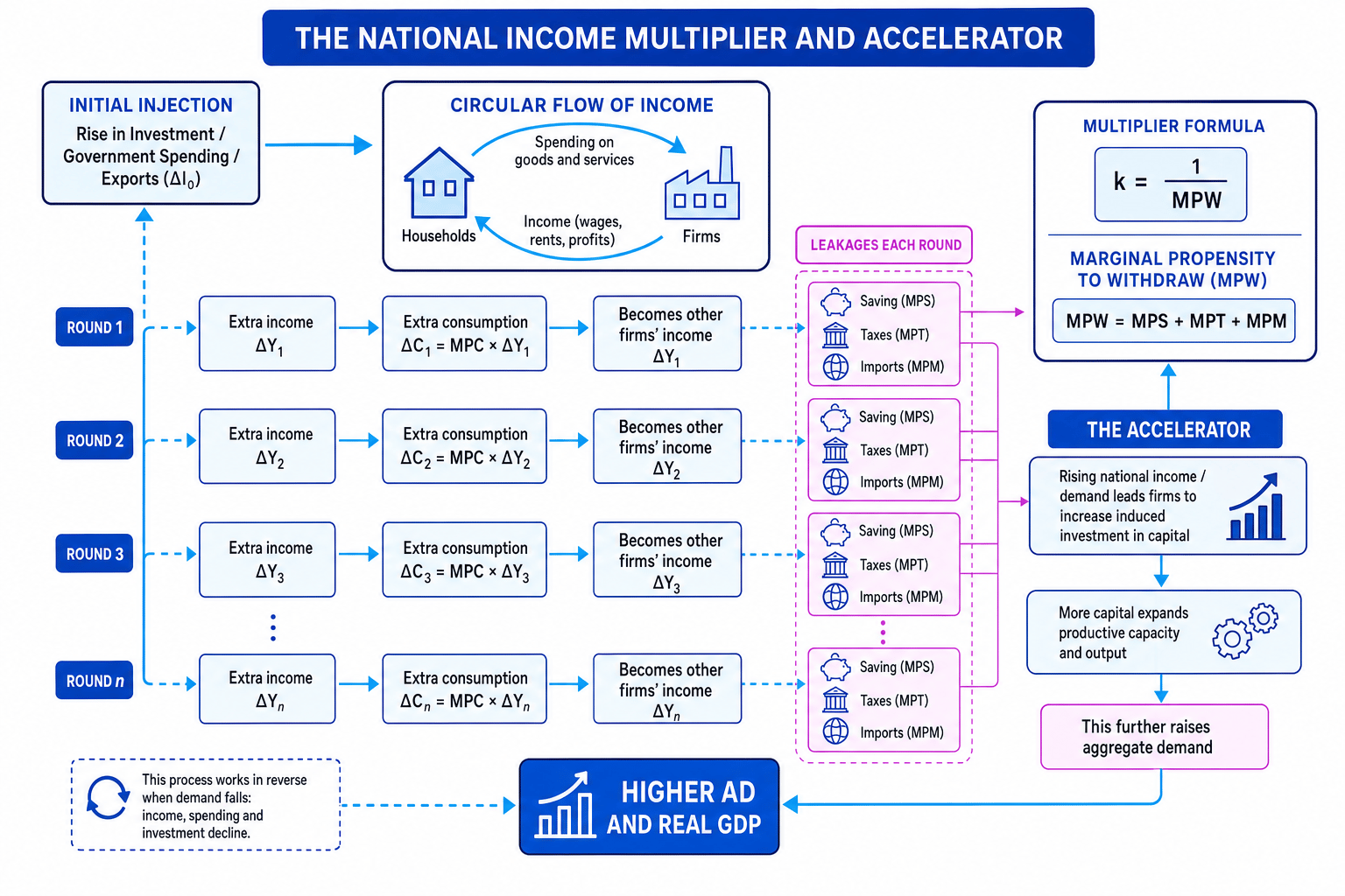
MPW=MPS+MPT+MPM\text{MPW} = \text{MPS} + \text{MPT} + \text{MPM}

Here, MPT is the marginal propensity to tax and MPM is the marginal propensity to import.

In the simple model, each extra £1 of income is either consumed or withdrawn, so:

MPC+MPW=1\text{MPC} + \text{MPW} = 1

Example

Calculating propensities

National income rises from £1,000bn to £1,080bn. Consumption rises from £650bn to £706bn, saving rises from £120bn to £132bn, and total withdrawals rise from £350bn to £374bn.

Calculate average propensities using the new total income: $APC=7061080≈0.654\text{APC} = \frac{706}{1080} \approx 0.654$ , $APS=1321080≈0.122\text{APS} = \frac{132}{1080} \approx 0.122$ , and $APW=3741080≈0.346\text{APW} = \frac{374}{1080} \approx 0.346$ .
Calculate the changes: $ΔY=80\Delta Y = 80$ , $ΔC=56\Delta C = 56$ , $ΔS=12\Delta S = 12$ , and $ΔW=24\Delta W = 24$ , all in £bn.
Calculate marginal propensities: $MPC=5680=0.70\text{MPC} = \frac{56}{80} = 0.70$ , $MPS=1280=0.15\text{MPS} = \frac{12}{80} = 0.15$ , and $MPW=2480=0.30\text{MPW} = \frac{24}{80} = 0.30$ .
Check the logic: $MPC+MPW=0.70+0.30=1.00\text{MPC} + \text{MPW} = 0.70 + 0.30 = 1.00$ , so the extra income has been fully accounted for.

Common Mistake

Average is not marginal

Do not use total consumption to calculate MPC. APC uses total income; MPC uses the change in consumption divided by the change in income.

The national income multiplier

Definition

National income multiplier

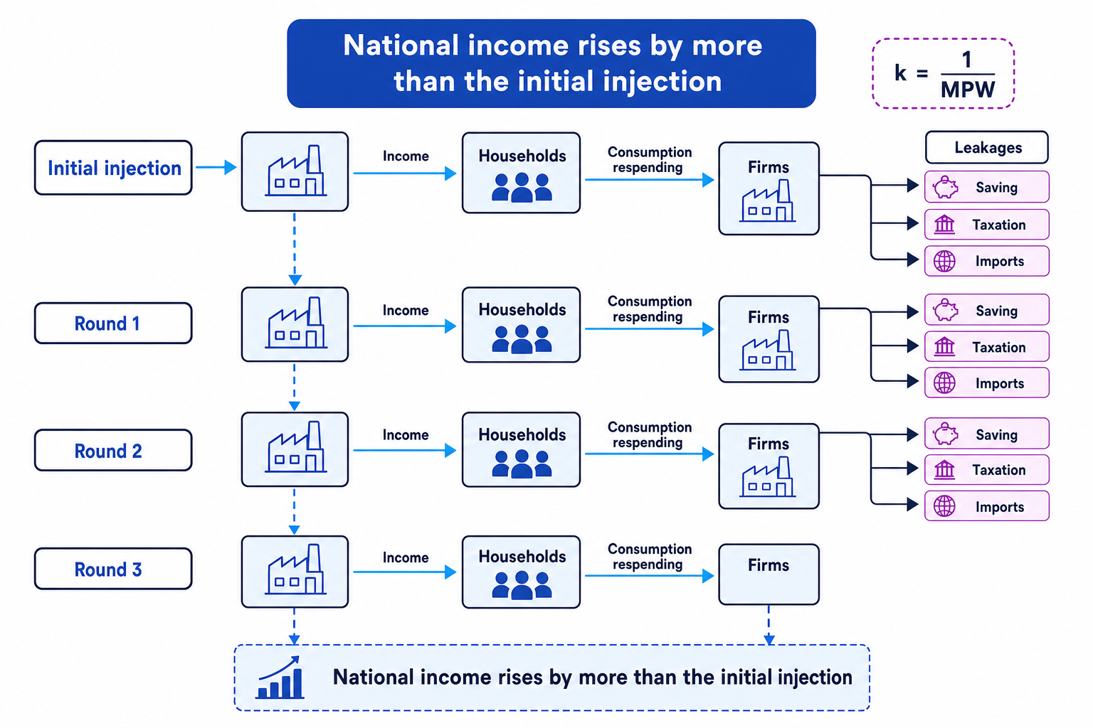
The national income multiplier is the process by which an initial change in an injection causes a larger final change in national income. The multiplier is $\frac{1}{\text{MPW}}$ , so the final change is $ΔY=k×ΔJ\Delta Y = k \times \Delta J$ , where $ΔJ\Delta J$ is the initial change in injections.

The logic is Keynesian: one person’s spending becomes another person’s income. If households spend part of that extra income, firms receive more revenue, workers receive more income, and further rounds of spending follow.

Diagram showing the national income multiplier, leakages and the accelerator

Example

Calculating the multiplier effect

Suppose government capital spending rises by £18bn. The marginal propensity to save is 0.10, the marginal propensity to tax is 0.15, and the marginal propensity to import is 0.05.

Add the marginal withdrawals: $MPW=0.10+0.15+0.05=0.30\text{MPW} = 0.10 + 0.15 + 0.05 = 0.30$ .
Calculate the multiplier: $\frac{1}{0.30} \approx 3.33$ .
Apply the multiplier to the injection: $ΔY=3.33×£18bn≈£60bn\Delta Y = 3.33 \times £18\text{bn} \approx £60\text{bn}$ .
Interpret the result: if there is spare capacity, real GDP may rise by about £60bn; if the economy is near full capacity, more of the effect may appear as higher prices instead.

What determines the size of the multiplier?

Key Idea

Small leakages mean a bigger multiplier

The multiplier is larger when more of each extra £1 is re-spent on domestic output, and smaller when the extra income is saved, taxed or spent on imports.

The main factors are:

MPC: a higher marginal propensity to consume means more re-spending, so a larger multiplier.
MPS: more saving reduces the next round of spending.
Taxation: higher marginal tax rates reduce disposable income, lowering consumption.
Imports: if consumers spend extra income on imports, demand leaks abroad. This matters for the UK because many consumer goods, energy products and intermediate inputs are imported.
Spare capacity: if firms have unused workers, machines and premises, extra demand can raise output. Near full capacity, extra AD may mainly raise inflation.
Confidence and credit conditions: during a cost-of-living squeeze or when Bank of England interest rates are high, households may save more or repay debt, weakening the multiplier.
Policy reactions: if fiscal stimulus causes inflationary pressure, the Bank of England may raise interest rates, partly offsetting the rise in AD.

The accelerator

Definition

Accelerator theory

The accelerator is the idea that investment depends on the rate of change of national income or demand. If firms need a higher capital stock to meet rising demand, they increase induced investment, which is investment caused by changes in output.

A simple accelerator relationship is:

Iinduced=v×ΔYI_{\text{induced}} = v \times \Delta Y

Here, $v$ is the capital-output ratio: the amount of capital needed to produce £1 of output.

Example

Applying the accelerator

Suppose firms need £2 of capital for every extra £1 of annual output, so $v = 2$ . Output rises from £100bn to £112bn, then rises again to £118bn.

For the first rise, $ΔY=£12bn\Delta Y = £12\text{bn}$ , so induced investment is $\times £12\text{bn} = £24\text{bn}$ .
For the second rise, $ΔY=£6bn\Delta Y = £6\text{bn}$ , so induced investment is $\times £6\text{bn} = £12\text{bn}$ .
Notice the key point: output is still rising, but induced investment has fallen from £24bn to £12bn because the growth of output has slowed.

Common Mistake

The accelerator is about changes in growth

High output alone does not guarantee rising investment. The accelerator says investment responds to the change in demand/output, so investment can fall even while GDP is still increasing.

Multiplier, accelerator and the economic cycle

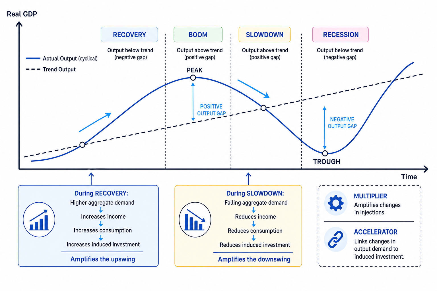
The economic cycle is the pattern of fluctuations in real GDP around its long-run trend. Typical phases are recovery, boom, slowdown and recession.

The multiplier and accelerator can reinforce each other:

A rise in injections shifts AD right.
The multiplier increases income and consumption over several rounds.
Rising demand encourages firms to invest, creating an accelerator effect.
That extra investment is itself a component of AD, so it can be multiplied again.

In a downturn, the same process works in reverse. Falling AD reduces income, consumption falls, firms cut investment, and the fall in investment further reduces AD. This is why investment is often one of the most volatile components of aggregate demand.

Economic cycle diagram showing multiplier and accelerator effects in recovery, boom, slowdown and recession

Common Mistake

Feedback can be dampened

The multiplier-accelerator process is not automatic or infinite. Leakages, weak confidence, limited credit, inventories, spare capacity limits and policy responses can all weaken the feedback loop.

Output gaps using AD-AS and the PPC

Definition

Output gap

An output gap is the difference between actual real GDP and potential output. Potential output, often shown as $Y^*$ , is the sustainable level of output when resources are normally employed.

The output gap can be expressed as:

(%)=Y−Y∗Y∗×100\text{Output gap (\%)} = \frac{Y - Y^*}{Y^*} \times 100

A negative output gap occurs when actual output is below potential output. There is spare capacity and cyclical unemployment.

A positive output gap occurs when actual output is above sustainable potential output. The economy is operating beyond normal capacity, creating inflationary pressure.

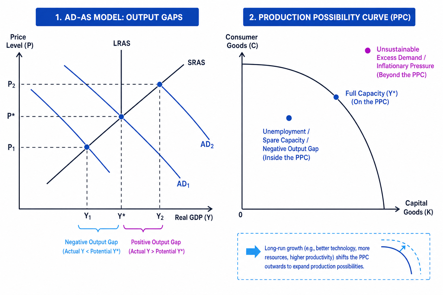
AD-AS and PPC diagrams showing negative and positive output gaps

In the AD-AS diagram, LRAS shows potential output. If AD is too low, equilibrium real GDP is left of LRAS, creating a negative output gap. If AD is too high, equilibrium is right of LRAS, creating a positive output gap.

In the PPC diagram, a point inside the PPC shows unemployed or underused resources, which links to a negative output gap. A point on the PPC shows full use of resources. A point beyond the PPC is not sustainable without inflationary pressure or long-run growth that shifts the PPC outwards.

Causes and consequences of output gaps

Causes of a negative output gap

A negative output gap is often caused by weak AD. For example, higher interest rates, falling real wages, lower consumer confidence, fiscal tightening or weaker exports can reduce spending. Recent UK examples include the cost-of-living squeeze reducing real disposable incomes and higher Bank of England interest rates weakening consumption and investment.

It can also reflect supply-side changes if potential output rises faster than actual demand, although in exams negative gaps are usually linked to deficient AD.

Consequences of a negative output gap

The main consequences are higher cyclical unemployment, lower profits, lower tax receipts and higher welfare spending. Inflationary pressure is usually weaker, and firms may delay investment.

A serious long-term risk is hysteresis, where short-run unemployment damages long-run productive potential because workers lose skills and firms reduce investment.

Causes of a positive output gap

A positive output gap can be caused by excessive AD, such as rapid credit growth, expansionary fiscal policy, strong export demand or a consumption boom.

It can also appear when potential output falls due to supply shocks. For example, global supply-chain disruption, energy price shocks, post-pandemic labour shortages or Brexit-related trade frictions may reduce the economy’s capacity, making existing AD more inflationary.

Consequences of a positive output gap

The main consequence is demand-pull inflation, often reinforced by wage pressure and bottlenecks. Imports may rise as domestic firms struggle to meet demand, worsening the current account. The central bank may respond with higher interest rates, which can reduce consumption and investment.

However, a mild positive gap may temporarily reduce unemployment and increase profits. If firms believe demand will be sustained, it may encourage investment and raise future capacity.

Evaluating output gaps

The impact of an output gap depends on its size, duration and cause.

A small negative gap may mainly reduce inflation without large unemployment costs. A large, persistent negative gap is much more damaging because it can cause long-term unemployment and lost productive capacity.

A positive output gap caused by strong demand may be manageable if productivity and investment are rising. But if it is caused by supply constraints, extra demand-side stimulus may worsen inflation without much extra output.

There is also a measurement issue: potential output is not directly observable. After shocks such as the pandemic, Brexit, energy price volatility or changes in labour force participation, economists may disagree about where $Y^*$ actually is.

Key Idea

Balanced judgement

Output gaps matter most when they are large and persistent. Negative gaps waste resources and risk hysteresis; positive gaps may boost short-run employment but can become inflationary if the economy is beyond sustainable capacity.

Exam technique

In the exam

Define the key term first: multiplier, accelerator or output gap, then link it clearly to AD and real GDP.
For calculations, carry £bn units through and check whether you need an average propensity or a marginal propensity.
For evaluation, judge whether the economy has spare capacity, how large the leakages are, and whether the shock is mainly demand-side or supply-side.

Self review

Check yourself

If MPW rises from 0.25 to 0.40, what happens to the size of the multiplier?
Why can investment fall even when national income is still rising?
How would a negative output gap appear on both an AD-AS diagram and a PPC?

What you'll learn

How injections, leakages and marginal propensities determine the national income multiplier.
How to calculate average and marginal propensities, plus the size of the multiplier.
Why the accelerator can make investment and the economic cycle more volatile.
How to explain and evaluate output gaps using AD-AS and PPC diagrams.

Start point: AD, income and the circular flow

Definition

Aggregate demand

So, an initial rise in government spending, exports or investment can cause a bigger final rise in national income — but only if enough of the extra income is re-spent rather than leaked away.

Average and marginal propensities

Definition

Average and marginal propensities

APC=CY,MPC=ΔCΔYAPS=SY,MPS=ΔSΔYAPW=WY,MPW=ΔWΔY\begin{aligned} \text{APC} &= \frac{C}{Y}, \quad \text{MPC} = \frac{\Delta C}{\Delta Y}\\ \text{APS} &= \frac{S}{Y}, \quad \text{MPS} = \frac{\Delta S}{\Delta Y}\\ \text{APW} &= \frac{W}{Y}, \quad \text{MPW} = \frac{\Delta W}{\Delta Y} \end{aligned}

The marginal propensity to withdraw (MPW) includes all marginal leakages:

MPW=MPS+MPT+MPM\text{MPW} = \text{MPS} + \text{MPT} + \text{MPM}

Here, MPT is the marginal propensity to tax and MPM is the marginal propensity to import.

In the simple model, each extra £1 of income is either consumed or withdrawn, so:

MPC+MPW=1\text{MPC} + \text{MPW} = 1

Example

Calculating propensities

National income rises from £1,000bn to £1,080bn. Consumption rises from £650bn to £706bn, saving rises from £120bn to £132bn, and total withdrawals rise from £350bn to £374bn.

Calculate average propensities using the new total income: $APC=7061080≈0.654\text{APC} = \frac{706}{1080} \approx 0.654$ , $APS=1321080≈0.122\text{APS} = \frac{132}{1080} \approx 0.122$ , and $APW=3741080≈0.346\text{APW} = \frac{374}{1080} \approx 0.346$ .
Calculate the changes: $ΔY=80\Delta Y = 80$ , $ΔC=56\Delta C = 56$ , $ΔS=12\Delta S = 12$ , and $ΔW=24\Delta W = 24$ , all in £bn.
Calculate marginal propensities: $MPC=5680=0.70\text{MPC} = \frac{56}{80} = 0.70$ , $MPS=1280=0.15\text{MPS} = \frac{12}{80} = 0.15$ , and $MPW=2480=0.30\text{MPW} = \frac{24}{80} = 0.30$ .
Check the logic: $MPC+MPW=0.70+0.30=1.00\text{MPC} + \text{MPW} = 0.70 + 0.30 = 1.00$ , so the extra income has been fully accounted for.

Common Mistake

Average is not marginal

Do not use total consumption to calculate MPC. APC uses total income; MPC uses the change in consumption divided by the change in income.

The national income multiplier

Definition

National income multiplier

Diagram showing the national income multiplier, leakages and the accelerator

Example

Calculating the multiplier effect

Suppose government capital spending rises by £18bn. The marginal propensity to save is 0.10, the marginal propensity to tax is 0.15, and the marginal propensity to import is 0.05.

Add the marginal withdrawals: $MPW=0.10+0.15+0.05=0.30\text{MPW} = 0.10 + 0.15 + 0.05 = 0.30$ .
Calculate the multiplier: $\frac{1}{0.30} \approx 3.33$ .
Apply the multiplier to the injection: $ΔY=3.33×£18bn≈£60bn\Delta Y = 3.33 \times £18\text{bn} \approx £60\text{bn}$ .
Interpret the result: if there is spare capacity, real GDP may rise by about £60bn; if the economy is near full capacity, more of the effect may appear as higher prices instead.

What determines the size of the multiplier?

Key Idea

Small leakages mean a bigger multiplier

The multiplier is larger when more of each extra £1 is re-spent on domestic output, and smaller when the extra income is saved, taxed or spent on imports.

The main factors are:

MPC: a higher marginal propensity to consume means more re-spending, so a larger multiplier.
MPS: more saving reduces the next round of spending.
Taxation: higher marginal tax rates reduce disposable income, lowering consumption.
Imports: if consumers spend extra income on imports, demand leaks abroad. This matters for the UK because many consumer goods, energy products and intermediate inputs are imported.
Spare capacity: if firms have unused workers, machines and premises, extra demand can raise output. Near full capacity, extra AD may mainly raise inflation.
Confidence and credit conditions: during a cost-of-living squeeze or when Bank of England interest rates are high, households may save more or repay debt, weakening the multiplier.
Policy reactions: if fiscal stimulus causes inflationary pressure, the Bank of England may raise interest rates, partly offsetting the rise in AD.

The accelerator

Definition

Accelerator theory

A simple accelerator relationship is:

Iinduced=v×ΔYI_{\text{induced}} = v \times \Delta Y

Here, $v$ is the capital-output ratio: the amount of capital needed to produce £1 of output.

Example

Applying the accelerator

Suppose firms need £2 of capital for every extra £1 of annual output, so $v = 2$ . Output rises from £100bn to £112bn, then rises again to £118bn.

For the first rise, $ΔY=£12bn\Delta Y = £12\text{bn}$ , so induced investment is $\times £12\text{bn} = £24\text{bn}$ .
For the second rise, $ΔY=£6bn\Delta Y = £6\text{bn}$ , so induced investment is $\times £6\text{bn} = £12\text{bn}$ .
Notice the key point: output is still rising, but induced investment has fallen from £24bn to £12bn because the growth of output has slowed.

Common Mistake

The accelerator is about changes in growth

High output alone does not guarantee rising investment. The accelerator says investment responds to the change in demand/output, so investment can fall even while GDP is still increasing.

Multiplier, accelerator and the economic cycle

The economic cycle is the pattern of fluctuations in real GDP around its long-run trend. Typical phases are recovery, boom, slowdown and recession.

The multiplier and accelerator can reinforce each other:

A rise in injections shifts AD right.
The multiplier increases income and consumption over several rounds.
Rising demand encourages firms to invest, creating an accelerator effect.
That extra investment is itself a component of AD, so it can be multiplied again.

Economic cycle diagram showing multiplier and accelerator effects in recovery, boom, slowdown and recession

Common Mistake

Feedback can be dampened

The multiplier-accelerator process is not automatic or infinite. Leakages, weak confidence, limited credit, inventories, spare capacity limits and policy responses can all weaken the feedback loop.

Output gaps using AD-AS and the PPC

Definition

Output gap

An output gap is the difference between actual real GDP and potential output. Potential output, often shown as $Y^*$ , is the sustainable level of output when resources are normally employed.

The output gap can be expressed as:

(%)=Y−Y∗Y∗×100\text{Output gap (\%)} = \frac{Y - Y^*}{Y^*} \times 100

A negative output gap occurs when actual output is below potential output. There is spare capacity and cyclical unemployment.

A positive output gap occurs when actual output is above sustainable potential output. The economy is operating beyond normal capacity, creating inflationary pressure.

AD-AS and PPC diagrams showing negative and positive output gaps