Costs and economies of scale
What you'll learn
- How to explain and calculate fixed, variable, total, average and marginal costs.
- Why the short run can create the law of diminishing returns.
- How economies and diseconomies of scale affect long-run average costs.
- Why minimum efficient scale matters for business objectives and market structure.
Why costs matter for business objectives
Costs are central to business decisions. A firm trying to maximise profit, survive during a cost-of-living squeeze, expand market share, or compete on price must understand how its costs behave as output changes.
A firm’s costs also affect consumers and markets. If large firms achieve lower average costs, they may offer lower prices — but they may also gain market power and create barriers to entry.
Core cost terms
Production costs
A production cost is the monetary value of resources used to produce goods or services. These resources include labour, raw materials, energy, rent, machinery and finance.
Fixed and variable costs
A fixed cost is a cost that does not change with output in the short run. Examples include factory rent, insurance, business rates, or some salaried management costs.
A variable cost changes directly with output. Examples include raw materials, packaging, hourly wages linked to production, and energy used by machinery.
Total, average and marginal costs
Total fixed cost (TFC) is all fixed costs added together. Total variable cost (TVC) is all variable costs added together. Total cost (TC) is the full cost of producing a given level of output.
If QQQ means output, the key formulae are:
TC=TFC+TVCAC=TCQAFC=TFCQAVC=TVCQMC=ΔTCΔQ\begin{aligned} TC &= TFC + TVC \\ AC &= \frac{TC}{Q} \\ AFC &= \frac{TFC}{Q} \\ AVC &= \frac{TVC}{Q} \\ MC &= \frac{\Delta TC}{\Delta Q} \end{aligned}TCACAFCAVCMC=TFC+TVC=QTC=QTFC=QTVC=ΔQΔTCAverage cost (AC) means cost per unit of output. It is sometimes called average total cost.
Marginal cost (MC) means the extra cost of producing additional output. If output rises by more than one unit, MC is the average extra cost across that output change.
Calculating average and marginal cost
A food producer has daily fixed costs of £900. At 200 ready meals, variable costs are £1,100. At 260 ready meals, variable costs are £1,340. All cost figures in the calculation are in pounds.
- Calculate total cost at 200 meals: TC=900+1100=2000TC = 900 + 1100 = 2000TC=900+1100=2000, so total cost is £2,000.
- Calculate average cost at 200 meals: AC=2000200=10AC = \frac{2000}{200} = 10AC=2002000=10, so average cost is £10 per meal.
- Calculate total cost at 260 meals: TC=900+1340=2240TC = 900 + 1340 = 2240TC=900+1340=2240, so total cost is £2,240. The change in total cost is £240.
- Calculate marginal cost over the extra 60 meals: MC=24060=4MC = \frac{240}{60} = 4MC=60240=4, so marginal cost is £4 per additional meal.
Average cost is not marginal cost
Do not assume that if average cost is £10, the next unit also costs £10 to make. Average cost spreads total cost across all output; marginal cost focuses only on the extra cost caused by extra output.
Short run and long run
Short run and long run
The short run is a period in which at least one factor of production is fixed. The long run is a period in which all factors of production can be varied.
This is not about a fixed number of weeks or months. It depends on the industry.
For a café, the short run might mean the building and kitchen size are fixed, but staff hours and ingredients can change. For an electricity company, the short run could last much longer because building new generation capacity takes years.
A fixed factor is an input that cannot be changed in the short run, such as factory size. A variable factor is an input that can be changed, such as labour hours or raw materials.
The law of diminishing returns
Law of diminishing returns
The law of diminishing returns states that, in the short run, as more units of a variable factor are added to a fixed factor, the extra output from each additional unit of the variable factor will eventually fall.
The “extra output” from one more worker or machine hour is called marginal product.
The diagram shows a fixed amount of capital, such as a factory or oven, combined with increasing labour. At first, extra workers may specialise and raise marginal product. Eventually, the fixed factor becomes overcrowded, so each extra worker adds less output.
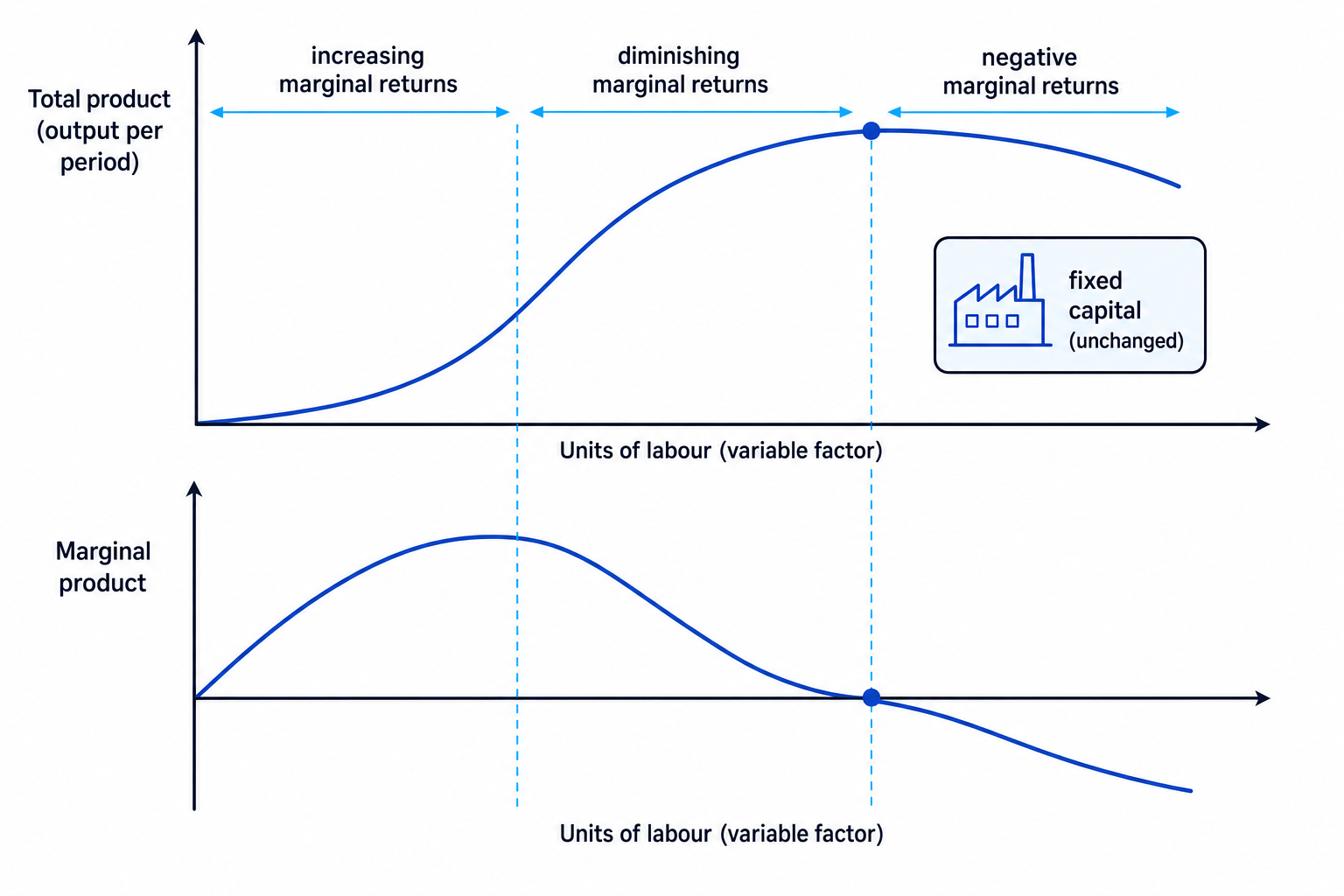
The key cost link is: when marginal product falls, marginal cost tends to rise. If each extra worker adds fewer units of output, the labour cost per extra unit produced increases.
Spotting diminishing returns
A bakery has one fixed oven. Each worker costs £80 per day. The first four workers produce total output of 40, 90, 125 and 150 cakes.
- Calculate marginal product: worker 1 adds 40 cakes, worker 2 adds 50 cakes, worker 3 adds 35 cakes, and worker 4 adds 25 cakes.
- Identify where diminishing returns begin: after worker 2, marginal product falls from 50 to 35, then to 25.
- Link this to marginal cost: worker 2 costs £80 and adds 50 cakes, so extra labour cost is £1.60 per extra cake. Worker 4 costs £80 and adds only 25 cakes, so extra labour cost is £3.20 per extra cake.
- Conclude that the fixed oven is becoming a constraint, causing falling marginal product and rising marginal cost.
Diminishing returns is short run only
Do not confuse diminishing returns with diseconomies of scale. Diminishing returns happen in the short run because at least one factor is fixed. Diseconomies of scale happen in the long run when the firm becomes too large and average cost rises.
Long-run average cost and economies of scale
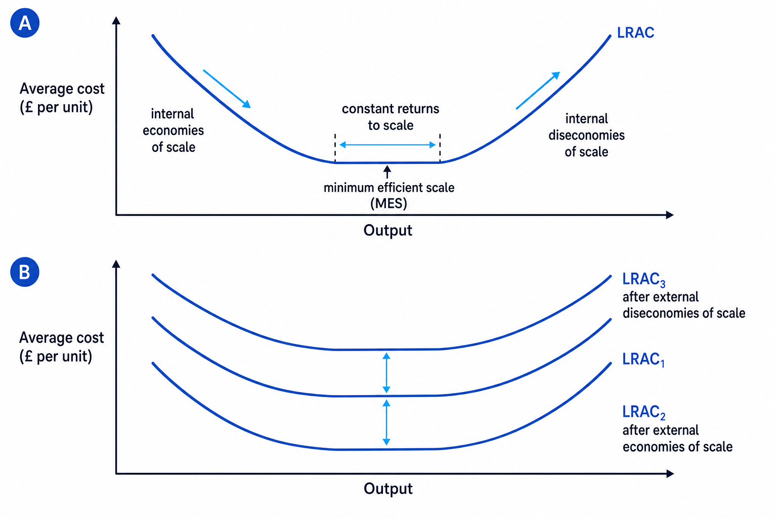
The long-run average cost (LRAC) curve shows the lowest possible average cost at each level of output when all factors of production can be varied.
Economies and diseconomies of scale
Economies of scale occur when long-run average cost falls as output increases. Diseconomies of scale occur when long-run average cost rises as output increases.
The diagram below is vital for OCR. Panel A shows internal economies and diseconomies as movements along the LRAC curve. Panel B shows external economies and diseconomies as shifts of the whole LRAC curve.
Internal economies of scale
Internal economies of scale are cost advantages gained from the growth of the individual firm.
Common causes include:
- Purchasing economies: large firms may buy inputs in bulk at lower unit prices.
- Technical economies: expensive machinery can be used more efficiently at high output.
- Managerial economies: specialists can manage finance, marketing, HR and logistics more effectively.
- Financial economies: large firms may borrow at lower interest rates because banks see them as less risky.
- Marketing economies: advertising costs can be spread across more units sold.
- Risk-bearing economies: large firms may diversify across products or regions.
External economies of scale
External economies of scale are cost advantages gained from the growth of the whole industry or local cluster, not just one firm.
For example, the growth of a UK technology cluster may attract skilled workers, specialist suppliers, training providers and better infrastructure. This can lower costs for all firms in that area.
Diseconomies of scale
Diseconomies occur when growth makes the firm or industry less efficient.
Internal causes include communication problems, bureaucracy, slower decision-making, weaker worker motivation, and principal-agent problems where managers pursue their own objectives rather than owners’ objectives.
External diseconomies can include congestion, higher local rents, competition for skilled labour, and pressure on transport or energy infrastructure.
Judging scale effects
A UK battery producer considers expanding output from 200,000 to 400,000 battery packs per year. It expects LRAC to fall from £4,800 to £4,200 per pack, but managers warn that coordination problems may appear above 450,000 packs.
- Identify the scale effect: the fall in LRAC as the firm expands is an internal economy of scale, likely from technical, purchasing and managerial economies.
- Calculate the unit saving: £4,800 minus £4,200 gives £600 saved per pack.
- Estimate the total potential saving at the new output: 600×400000=240000000600 \times 400000 = 240000000600×400000=240000000, so the saving is £240 million per year.
- Evaluate the risk: diseconomies are forecast above 450,000 packs, so expansion to 400,000 looks beneficial if demand exists and supply chains are reliable.
Minimum efficient scale
Minimum efficient scale (MES) is the lowest level of output at which LRAC is minimised. After this point, the firm has exhausted the available economies of scale.
If the LRAC curve has a flat bottom, MES is the start of the flat section, not the middle.
MES and market structure
If MES is very high relative to total market demand, only one or a few firms may be able to produce efficiently. This can lead to oligopoly or even natural monopoly. If MES is low, many small firms can survive at efficient scale.
Evaluating significance
Economies and diseconomies of scale are most significant in industries with high fixed costs and large potential output, such as car manufacturing, energy networks, airlines, supermarkets and digital platforms. Spreading fixed costs across more output can sharply reduce average cost.
However, their significance is lower where production is personalised, labour-intensive or quality-sensitive. A small legal practice, restaurant or design studio may compete successfully without huge scale because flexibility, service quality and reputation matter more than low unit cost.
The impact also depends on whether cost savings are passed on to consumers. A firm with strong market power may keep lower costs as higher profit rather than reducing prices. This links costs to competition policy and business objectives.
Evaluation judgement
The significance of economies and diseconomies of scale depends on the industry’s cost structure, the size of market demand, management quality, technology, and the time period considered. Bigger is not automatically better: scale can reduce costs, but excessive size can create inefficiency and market power.
In the exam
- Define the relevant cost or scale term precisely, and state whether you are analysing the short run or the long run.
- For calculations, write the formula, substitute the figures with units, and interpret whether the answer is total, per unit, or marginal.
- For diagrams, show movements along LRAC for internal scale effects and shifts of LRAC for external scale effects, then add a judgement about significance.
Check yourself
- A firm’s TFC is £500 and TVC is £1,500 at output 100. What is average cost?
- Why does diminishing marginal product tend to raise marginal cost?
- If MES is very high relative to total market demand, what might happen to market structure?