Aggregate demand

Welcome to macroeconomics! At its core, macroeconomics is about looking at the economy as a whole. Just as we use demand in microeconomics to study individual markets, we use Aggregate Demand (AD) to study the total demand for all goods and services within an economy.

---

What you'll learn

• The definition of Aggregate Demand and the formula used to calculate it.
• Why the AD curve slopes downward and what causes it to shift.
• How changes in disposable income affect consumer spending (using the Marginal Propensity to Consume).
• The vital role of consumer and business expectations in driving economic activity.

---

What is Aggregate Demand?

Unlike microeconomic demand, which looks at the quantity of a single good demanded at different prices, aggregate demand represents the total spending of the entire economy.

The Components of Aggregate Demand

To calculate Aggregate Demand, we sum the spending of four major macroeconomic sectors: households, firms, the government, and the international sector.

The fundamental formula is:

$$AD=C+I+G+(X-M)$$

Let's break down each of these components:

• Consumption ($C$): Spending by domestic households on goods and services (e.g., food, cars, haircuts). This is the largest component of UK aggregate demand, typically accounting for 60% to 65% of the total.
• Investment ($I$): Spending by private-sector firms on capital goods (such as machinery, technology, factories, and new offices) used to produce future goods and services. Note that in economics, "investment" does not mean buying stocks or bonds; it means physical capital accumulation. It accounts for about 15% of UK AD but is highly volatile.
• Government Spending ($G$): Spending by central and local government on state-provided goods and services (e.g., the NHS, state schools, defense, and infrastructure). It represents approximately 20% to 25% of UK AD.
• Net Exports ($X-M$): The value of domestic exports sold to foreign buyers ($X$) minus the value of foreign imports bought by domestic buyers ($M$). Because the UK historically imports more than it exports, the UK usually runs a trade deficit, making this a negative net contribution to AD (around -2% to -5%).

---

The Aggregate Demand Curve

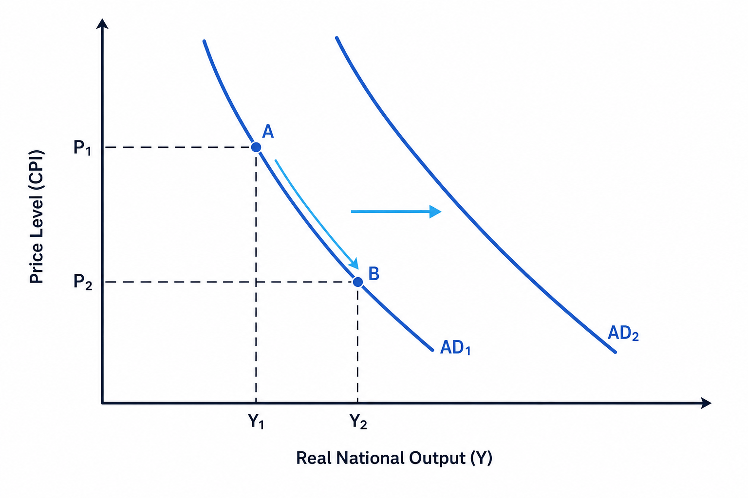
When we plot Aggregate Demand against the general price level (usually measured by the Consumer Prices Index, or CPI), we get a downward-sloping curve.

Why does the AD curve slope downward?

As the price level falls from $P_1$ to $P_2$, the real national output demanded expands from $Y_1$ to $Y_2$. This downward slope is explained by three key macroeconomic wealth and monetary effects:

1. The Wealth Effect (Pigou Effect): As the price level falls, the money in people's pockets and bank accounts has greater purchasing power. Households feel richer in real terms, leading them to increase their consumption spending ($C$).
2. The Interest Rate Effect (Keynesian Effect): When the price level is low, households need less cash to make daily transactions. This reduces the demand for money, which pushes down nominal interest rates. Lower interest rates reduce the cost of borrowing for households (mortgages, credit cards) and firms, stimulating both Consumption ($C$) and Investment ($I$).
3. The International Trade Effect: If the UK price level falls relative to other countries, UK exports become cheaper and more competitive abroad, increasing export volume ($X$). Concurrently, foreign imports become relatively more expensive to UK consumers, decreasing import volume ($M$). Both of these forces improve the net trade balance ($X-M$), expanding AD.

Movements vs. Shifts of the AD Curve

Just like in microeconomics, you must distinguish between a movement along the curve and a shift of the curve.

• Movements along the AD curve: A change in the price level causes a movement along the AD curve (from point A to point B in the diagram above). If the price level rises, AD contracts; if the price level falls, AD expands.
• Shifts of the AD curve: A change in any non-price factor that influences $C$, $I$, $G$, or $X-M$ will shift the entire AD curve. For example, a surge in consumer confidence or an expansionary fiscal policy (cutting income tax) shifts the curve rightwards from $A{D}_1$ to $A{D}_2$.

---

Evaluating Income and Consumption

Disposable income ($Y_d$) is the single most important determinant of household consumption. This is the income left over after paying direct taxes (such as income tax and National Insurance) and receiving state benefits.

The formula for the MPC is:

$$MPC=\frac{\Delta C}{\Delta Y_d}$$

Where $\Delta C$ is the change in consumption and $\Delta Y_d$ is the change in disposable income.

Similarly, the Average Propensity to Consume (APC) measures the fraction of total disposable income spent on consumption:

$$APC=\frac{C}{Y_d}$$

Evaluative Analysis: Income vs. Consumption

While consumption generally rises with income, you must evaluate how this relationship behaves across different economic contexts:

• Income distribution: Lower-income households have a much higher MPC (often close to 1.0) because they must spend almost all of any extra income on immediate necessities like food, rent, and heating. Wealthier households have a much lower MPC (and higher marginal propensity to save, MPS) because their basic needs are already met.
• The Keynesian Consumption Function: John Maynard Keynes argued that as real national income increases, aggregate consumption increases, but by a smaller amount. Thus, as an economy grows richer, its national saving rate tends to rise, which can lead to a deficiency in AD if those savings are not successfully channeled into investment.
• Temporary vs. Permanent Income changes (Friedman's Theory): If households believe an increase in income is only temporary (e.g., a one-off tax rebate or bonus), their MPC will be low. However, if they expect a permanent rise in income (e.g., a promotion or long-term tax cut), their MPC will be high. This makes the design of government fiscal policy highly sensitive to how households perceive tax changes.

---

Evaluating the Role of Expectations

Traditional economic models often treat consumers and firms as rational calculators responding purely to prices and interest rates. However, modern macroeconomics recognizes that expectations about the future play a dominant role in shifting Aggregate Demand.

1. Consumer Confidence

Consumer confidence reflects how optimistic households feel about their personal financial prospects and the broader economy.

• The Mechanism: If households expect interest rates to rise, house prices to crash, or unemployment to increase, they will proactively reduce discretionary consumption ($C$) and increase precautionary savings. This drags down AD, potentially triggering the very recession they feared (a self-fulfilling prophecy).
• The UK Context: During the post-pandemic recovery and the 2022–2023 cost-of-living squeeze, UK consumer confidence plummeted due to double-digit inflation and rising mortgage rates (with the Bank of England base rate climbing rapidly to 5.25%). This caused households to rein in spending on luxury items, illustrating how pessimistic expectations suppress AD even when unemployment remains low.

2. Business Confidence and "Animal Spirits"

The economist John Maynard Keynes coined the term "animal spirits" to describe the emotional waves of optimism and pessimism that influence financial markets and business investment decisions.

• The Mechanism: Investment ($I$) is highly risky and relies on predictions of future profitability. If firms have high business confidence, they will invest in new projects, expand production lines, and hire workers. If they are pessimistic, they will postpone or cancel projects, even if interest rates are extremely low.

---

---