1.4.5a Economies and diseconomies of scale
Economies of Scale Come from the Firm or the Industry
Definition
Economies of scale: the fall in long-run average cost that a firm experiences as it increases its scale of output.
- Internal economies of scale are cost advantages from a firm's own growth.
- External economies of scale are cost advantages from the growth of the whole industry.
- Diseconomies of scale are rising long-run average costs when a firm grows too large.
Note
- Internal economies come from the single firm expanding.
- External economies come from the whole industry expanding around it.
Where Internal Economies of Scale Come From
- Technical and purchasing
- Larger machines and bulk-buying discounts cut the cost per unit.
- Managerial and financial
- Specialist managers and cheaper borrowing lower average cost as the firm grows.
- Marketing and risk-bearing
- Advertising and a wide product range are spread over far more output.
Example
- A supermarket chain like Tesco secures deep bulk discounts from suppliers that a corner shop cannot match, cutting the cost per item.
- The spreading effect is easy to quantify: a £2 million advertising campaign spread over 1 million cars costs £2m1m=£2\dfrac{\pounds 2\text{m}}{1\text{m}} = \pounds 21m£2m=£2 per car, but over 4 million cars it is just £2m4m=£0.50\dfrac{\pounds 2\text{m}}{4\text{m}} = \pounds 0.504m£2m=£0.50 per car, so average cost falls purely from higher output.
- This is why large producers can often undercut smaller rivals on price.
Why Diseconomies of Scale Set In
- Internal diseconomies come from poor communication, weak coordination and lower motivation in a very large firm.
- External diseconomies come from congestion and rising input prices as the whole industry expands.
- These push long-run average cost back up once the firm grows too large.
How Returns to Scale Link to Economies of Scale
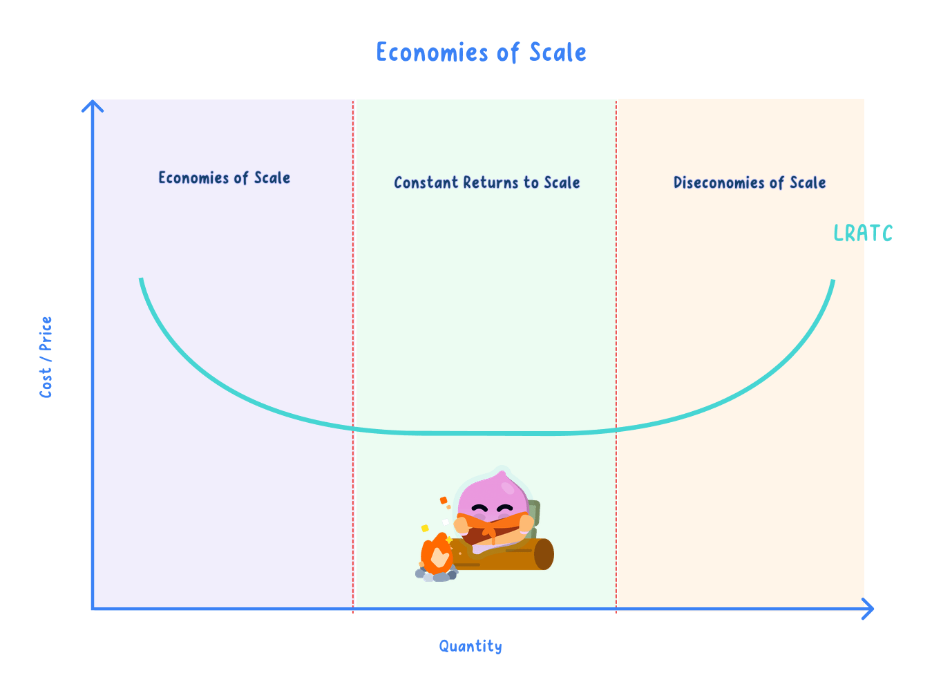
- Increasing returns to scale mean output rises more than in proportion to inputs, so long-run average cost falls: economies of scale.
- Decreasing returns to scale mean output rises less than in proportion, so long-run average cost rises: diseconomies of scale.
- Constant returns to scale leave long-run average cost unchanged.
How Scale Effects Shape the LRAC Curve
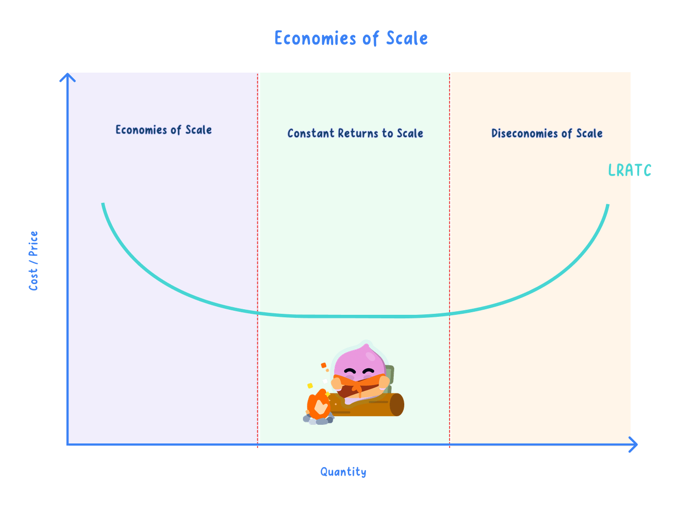
- Internal and external economies drive the falling section of the LRAC curve.
- Diseconomies drive the rising section as coordination becomes harder.
- Between them the curve reaches its lowest average cost.
Is Bigger Always Better?
- Growing larger can cut long-run average cost sharply through internal economies such as bulk-buying and specialist management, giving big firms a genuine price advantage.
- But once a firm grows past its optimum, diseconomies of scale set in as poor communication and weak coordination push long-run average cost back up.
- How far economies run depends on the industry, reaching very high output in capital-heavy sectors like car-making or utilities but being exhausted quickly in personal services.
- So bigger is better only up to a point, and whether further growth pays depends on where the firm sits on its LRAC curve relative to the balance between economies and diseconomies at that output.
Name the Type, Then the Source
Exam technique
- State whether an economy is internal or external before naming its source.
- Tie each effect to the falling or rising part of the LRAC curve.
Common Mistake
- Do not confuse internal economies with external economies.
- Do not confuse diseconomies of scale with short-run diminishing returns.
Self review
- Distinguish internal from external economies of scale.
- Name three internal economies of scale.
- Give two reasons for diseconomies of scale.
- How do increasing and decreasing returns to scale relate to economies and diseconomies of scale?
- Which parts of the LRAC curve do economies and diseconomies explain?
1.4.5b Long-run average cost and minimum efficient scale
The Long-Run Average Cost Curve Is the Envelope of Short-Run Curves
Definition
Long-run average cost (LRAC): the lowest average cost of producing each level of output when all factors of production can be varied.
Minimum efficient scale (MES): the lowest level of output at which a firm can produce so that long-run average cost is minimised.
- In the long run, all factors are variable.
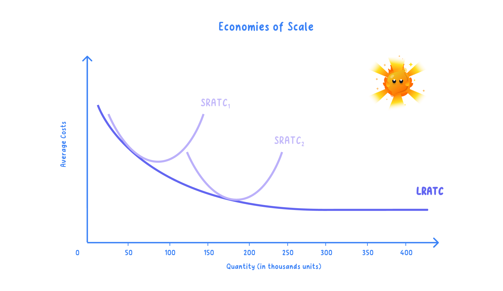
- The long-run average cost curve is built up as the envelope of the short-run curves.
- It is typically L-shaped or U-shaped.
Note
- Each short-run curve fits one scale of plant.
- The LRAC is tangent to each SRAC, tracing their lower envelope.
How the Short-Run and Long-Run Curves Relate
- Each SRAC shows costs for a fixed plant size.
- As the firm changes scale, it moves to a different SRAC.
- The LRAC is the lowest cost achievable at each output.
Example
- A small plant has low costs only at low output.
- A larger plant reaches lower costs at higher output.
What the Shape of the LRAC Tells You
- A falling LRAC section reflects economies of scale.
- A flat or rising section reflects constant returns or diseconomies of scale.
- An L-shaped LRAC falls steeply, then stays low and roughly flat as diseconomies remain small.
Draw the Envelope, Not a Join
Exam technique
- Draw the LRAC tangent to each SRAC curve.
- Link the falling section to economies of scale and any rising section to diseconomies.
Common Mistake
- Do not draw the LRAC joining the bottoms of the SRAC curves.
- It is their lower envelope, tangent to each.
Minimum Efficient Scale: The First Low-Cost Output
- Reaching the MES matters because it is the smallest size at which a firm's average cost is as low as its larger rivals'.
- On the curve, it is where average cost first stops falling.
- On an L-shaped LRAC, it is where cost first becomes constant.

Note
- At the MES the firm has captured all available economies of scale.
- Producing below it means paying higher average costs than rivals.
- A small MES relative to the market lets many firms compete.
- A large MES relative to the market supports only a few large firms.
- A high MES can act as a barrier to entry for newcomers.
Example
- Hairdressing has a low MES, perhaps a few chairs, so many small salons coexist in one town.
- Car manufacturing has a very high MES: if a plant must produce around 2 million cars a year to reach lowest cost while national demand is only a few million, just a handful of firms can fit, which is why the industry is concentrated.
Finding the MES on the LRAC Curve
- Trace the LRAC until it stops falling, and that output is the MES.
- To the left of it, firms are too small to be cost-competitive.
- To the right, average cost is flat or eventually rising.
Does a High MES Always Concentrate a Market?
- A high MES relative to demand does give large firms a real cost advantage and can leave room for only a few producers, as in car manufacturing.
- But the L-shaped LRAC means that beyond the MES extra size brings no further cost saving, so the very largest firm is not necessarily cheaper than a mid-sized rival already at the MES.
- Where the MES is small relative to the market, many firms can each reach lowest cost, so the industry can stay competitive.
- A high MES is only a cost-based barrier, not an absolute one, since new technology or a contestable market can lower it or let entrants compete.
- So MES shapes but does not dictate structure, and the deciding factor is the size of the MES relative to total market demand, alongside how fast technology is changing costs.
Compare MES to Market Size
Exam technique
- Judge the number of firms by comparing MES with total market demand.
- On an L-shaped curve, mark MES where cost first becomes constant.
Common Mistake
- Do not treat MES as a single lowest-cost point.
- With an L-shaped LRAC it is where average cost first becomes constant.
Self review
- Why is the LRAC the envelope of the SRAC curves?
- What do the falling, flat and rising sections of the LRAC show about economies and diseconomies of scale?
- Describe the L-shaped long-run average cost curve.
- Define minimum efficient scale.
- Why does a low MES support many firms, and how can a high MES act as a barrier to entry?
