The Phillips Curve
- The Phillips curve maps the rate of inflation against the rate of unemployment, capturing the central conflict between two key macro objectives.
- A demand-driven boom that cuts unemployment tends to raise inflation, so the short-run curve slopes downward.
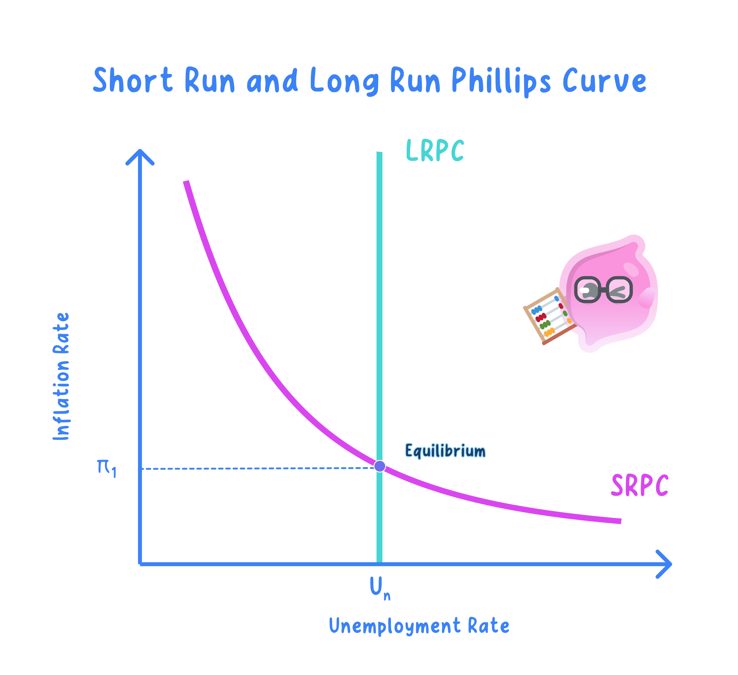
- Once workers adjust their inflation expectations the economy returns to the natural rate, so the long-run curve is vertical and offers no lasting trade-off.
- In the short run lower unemployment usually comes with higher inflation, giving policymakers a tempting trade-off.
- In the long run the economy settles at the natural rate of unemployment, so demand policy cannot buy a permanent fall in unemployment.
The Traditional Short-Run Curve
Phillips curve: the observed relationship between the rate of unemployment and the rate of inflation.
Traditional Phillips curve: the original single curve, sloping downward, that shows an inverse trade-off between unemployment and inflation.
- The rate of unemployment is measured on the horizontal axis and the rate of inflation on the vertical axis.
- The curve slopes downward because heavier demand for labour bids up wages and prices as spare capacity shrinks.
- A rise or fall in aggregate demand is shown as a movement along the curve, not a shift of it.
- Cause to effect: stronger demand raises output, firms hire more, unemployment falls, and the tighter labour market pushes pay and prices up.
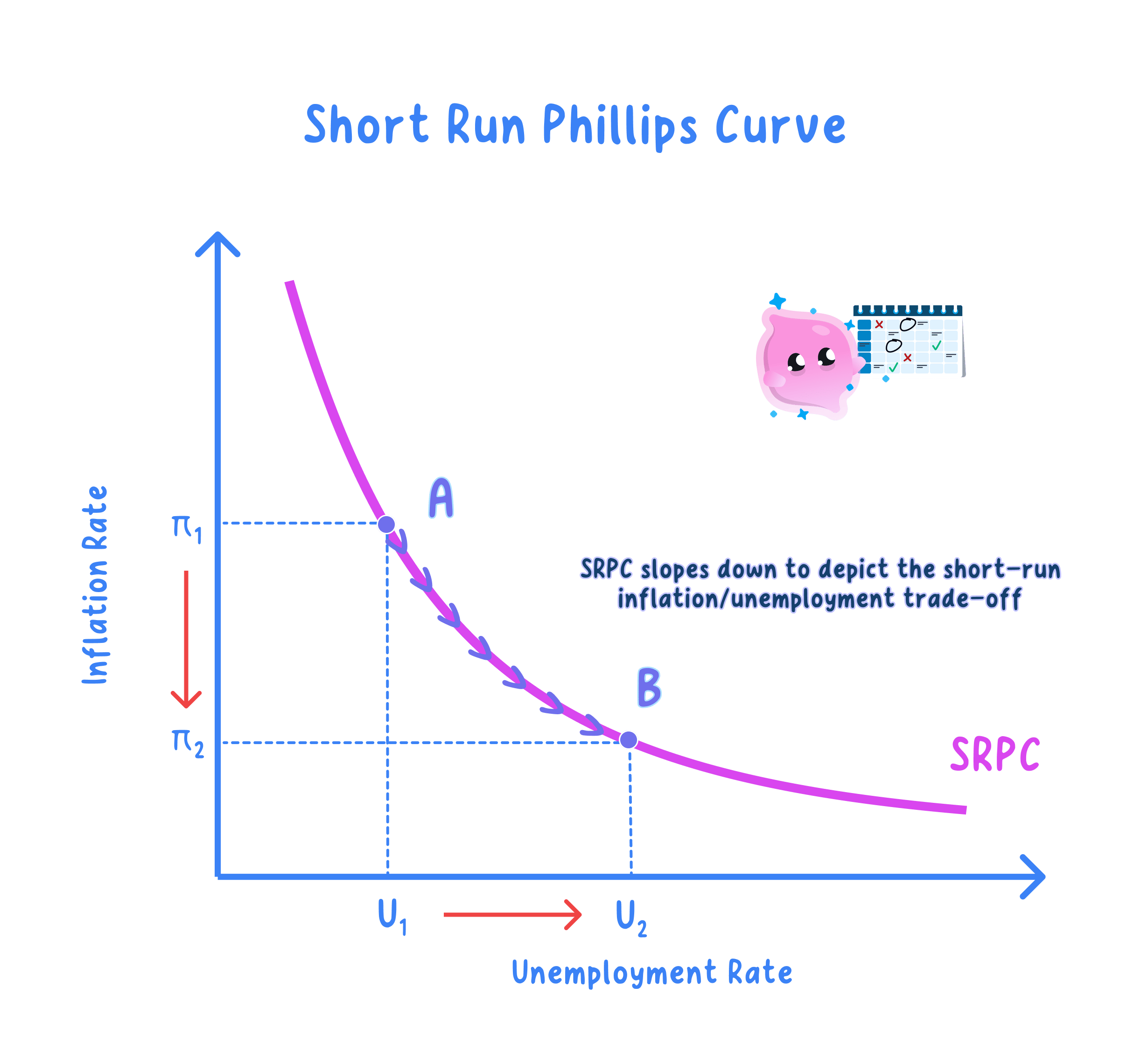
- Suppose unemployment sits at 5% with inflation at 2%.
- A spending boom lifts average weekly earnings from £600 to £640, so firms expand output and unemployment falls to 3%.
- The tighter labour market and stronger demand push inflation up to 4%, a movement up along the short-run curve.
- A later downturn that raises unemployment eases inflation back down, tracing the curve in reverse.
Linking to AD-AS and Output Gaps
- A rise in aggregate demand lowers unemployment as firms hire more workers to meet extra orders.
- The same rise adds to inflation as the economy nears full capacity and shortages appear.
- A positive output gap therefore lines up with low unemployment and higher inflation.
- A negative output gap lines up with high unemployment and low inflation.
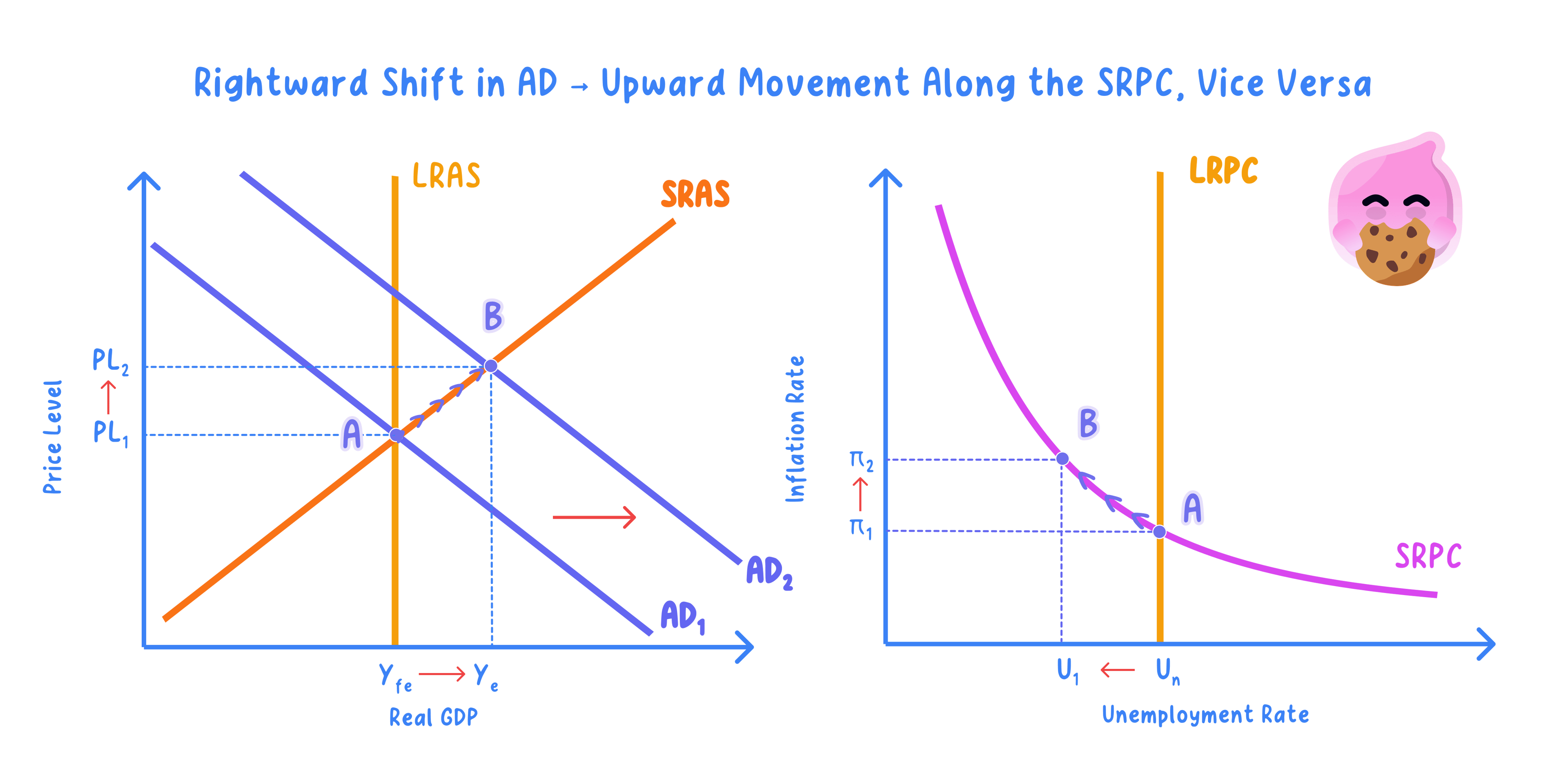
- The short-run Phillips curve is the labour-market counterpart of the AD-AS model.
- The apparent trade-off tempts governments to expand demand to cut unemployment while accepting higher inflation.
The Expectations-Augmented Curve
Expectations-augmented Phillips curve: a version that adds workers' expected inflation, giving a separate short-run curve for each expected rate.
Natural rate of unemployment: the equilibrium rate at which the labour market clears, made up of frictional and structural unemployment.
- Holding unemployment below the natural rate first raises inflation as demand outstrips supply.
- Workers then expect higher inflation and demand higher money wages to protect their real pay.
- Higher wage costs make firms cut hiring, so unemployment drifts back to the natural rate.
- The economy ends at the natural rate but with higher inflation, so the short-run curve has shifted up.
- Government stimulus cuts unemployment below the natural rate, lifting a worker's pay from £500 to £525 a week, a rise of +5%.
- Once workers expect 5% inflation they demand money-wage rises of at least +5% simply to keep real pay unchanged.
- These higher £ wage costs make firms shed labour, so unemployment returns to the natural rate at higher inflation.
- The short-run curve shifts upward to sit at the new, higher expected rate of inflation.
- Trying to hold unemployment below the natural rate gives accelerating inflation over time.
- Each short-run curve is drawn for one given expected rate of inflation.
The Long-Run Curve and the NAIRU
Short-run Phillips curve: a downward-sloping curve drawn for a given expected inflation rate, showing a temporary inverse trade-off.
Long-run Phillips curve: a vertical line at the natural rate of unemployment, showing no permanent trade-off.
NAIRU: the non-accelerating inflation rate of unemployment, the natural rate at which inflation stays stable.
- Cause to effect: expectations adjust, so any attempt to hold unemployment below the natural rate only accelerates inflation.
- At the natural rate the labour market clears, so a stable inflation rate can be sustained at any level.
- This natural rate is a supply-side equilibrium, not zero unemployment, since search and skills mismatch remain.
- Demand policy cannot cut unemployment below the NAIRU for long without accelerating inflation.
- Only supply-side change can move the natural rate itself.
Shifting the Long-Run Curve
- The natural rate depends on how well the labour market matches workers to jobs.
- Better skills and training cut structural unemployment by making workers employable in growing industries.
- Improved job-search information and stronger work incentives cut frictional unemployment.
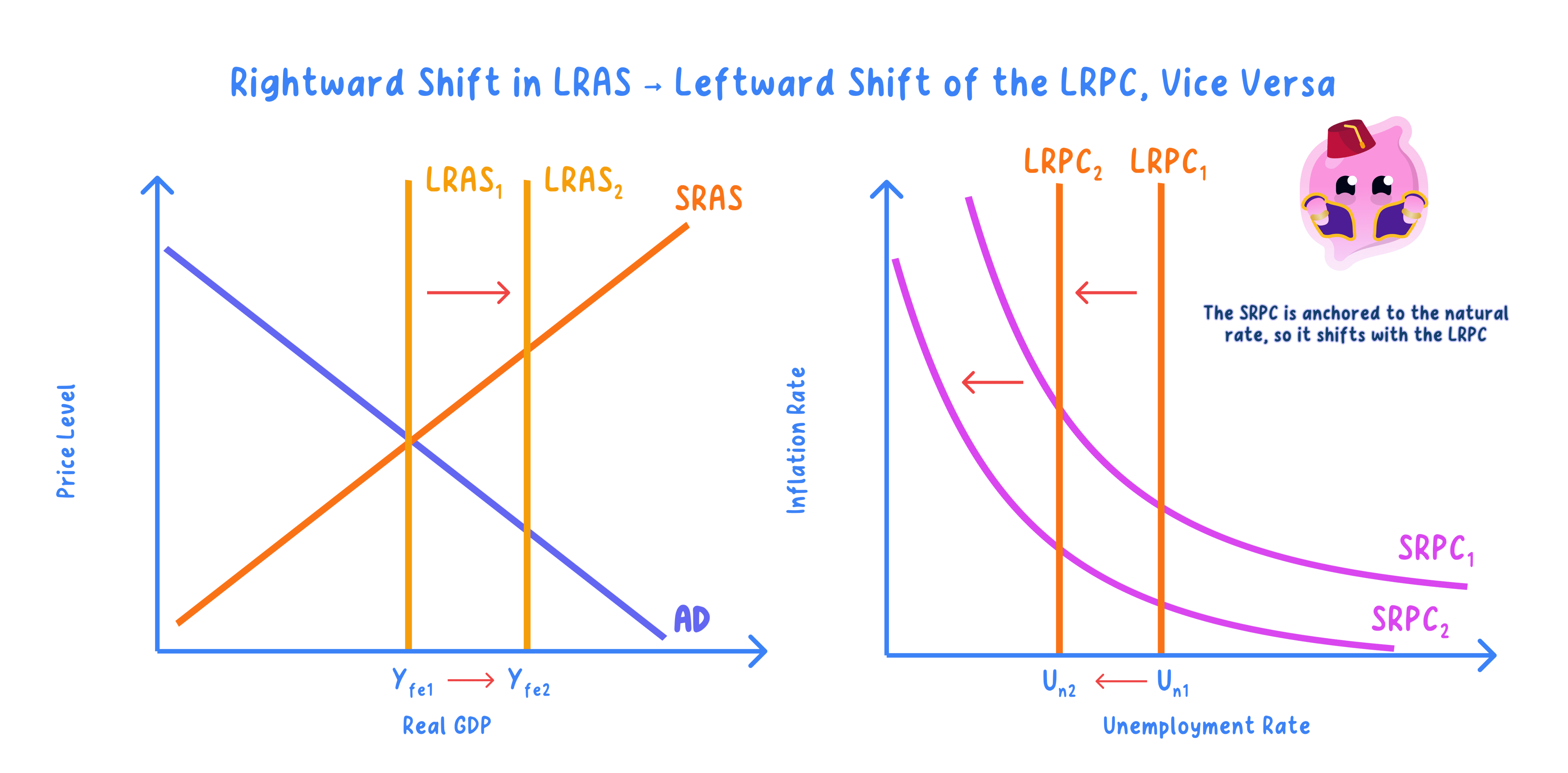
- These supply-side gains lower the natural rate and shift the long-run curve to the left.
- Suppose a £2bn retraining programme lifts the skills of the long-term unemployed.
- As structural unemployment falls the NAIRU drifts from about 6% towards 4%.
- The long-run curve shifts left, so lower unemployment can now coexist with a stable 2% inflation target.
Evaluation: Stagflation and Limits
- In the 1970s many economies suffered stagflation, with high inflation and high unemployment at the same time.
- Oil price shocks caused cost-push inflation while output fell, so both variables rose together and broke the simple stable trade-off.
- This experience pushed economists towards the expectations-augmented model and reshaped how central banks anchor inflation.
- The short-run curve stays a useful near-term guide, but expectations and the vertical long-run curve deny any lasting trade-off.
- It depends: supply-side reform can lower the natural rate, but it works slowly and the size of the effect is uncertain.
- How binding the short-run trade-off is also depends on credibility: when a central bank's inflation target is believed, expectations stay anchored and the short-run curve is flat, so a fall in unemployment brings only a small rise in inflation; when credibility is weak, expectations adjust fast and even a small fall in unemployment triggers sharply higher inflation, so the trade-off is barely usable.
- In the 1970s the oil price roughly quadrupled, adding sharply to firms' £ energy and transport costs.
- These higher £ costs forced firms to raise prices and cut output, so inflation and unemployment rose together.
- Across many economies, including the United States and the United Kingdom, inflation climbed into double figures while unemployment also rose, a mix the single downward-sloping curve could not explain.
- Cost-push shocks shift the short-run curve outward rather than move the economy along it.
- On balance the Phillips curve is a strong short-run guide but cannot deliver a permanent trade-off.
- Lasting falls in unemployment need supply-side reform rather than demand expansion.
- Draw the short-run curve downward sloping and the long-run curve vertical at the natural rate.
- Label unemployment on the horizontal axis and inflation on the vertical axis.
- Show a demand change as a movement along the short-run curve and a supply-side gain as a leftward shift of the long-run curve.
- Use inflation expectations and the 1970s stagflation to evaluate the trade-off.
- Do not treat the short-run trade-off as stable and permanent, because expectations and the long-run curve remove it.
- Do not confuse the natural rate with zero unemployment, since it includes frictional and structural unemployment.
- Do not use demand policy to explain a lower natural rate, because only supply-side change shifts the long-run curve.
- What does the traditional short-run Phillips curve show, and what are its axes?
- How do inflation expectations shift the short-run curve?
- Why is the long-run Phillips curve vertical at the NAIRU?
- What can shift the long-run curve to the left?
- How did 1970s stagflation challenge the traditional Phillips curve?
