What half-life means
Definition
Half-life
The half-life of a radioactive isotope is the time taken for half the undecayed nuclei in a sample to decay, or for the activity of a source to fall by half.
Definition
Undecayed nuclei
Undecayed nuclei are the nuclei in a sample that have not yet decayed at a given moment.
- Activity falls away smoothly towards zero, so there is no moment at which a source can be said to have finished decaying, and no way to quote a simple lifetime for it.
- Half-life solves this by timing the loss of a fixed fraction rather than a fixed amount, and the fraction chosen is one half.
- There are two equivalent statements of it, and either is acceptable.
- The time taken for half the undecayed nuclei in a sample to decay.
- The time taken for the activity of a source to fall to half its starting value.
- The two agree because activity is proportional to the number of undecayed nuclei, so halving one halves the other.
- Half-life is a time, so it is quoted in seconds, hours, days or years, and never as a fraction or a rate.
- Half-life is a property of the isotope, so every sample of the same isotope shares it, and it cannot be altered by heating, cooling, dissolving, compressing or chemically reacting the material.
- A short half-life means the activity dies away quickly, and a long half-life means a lower activity that persists for a very long time.
Half-life is constant along the curve
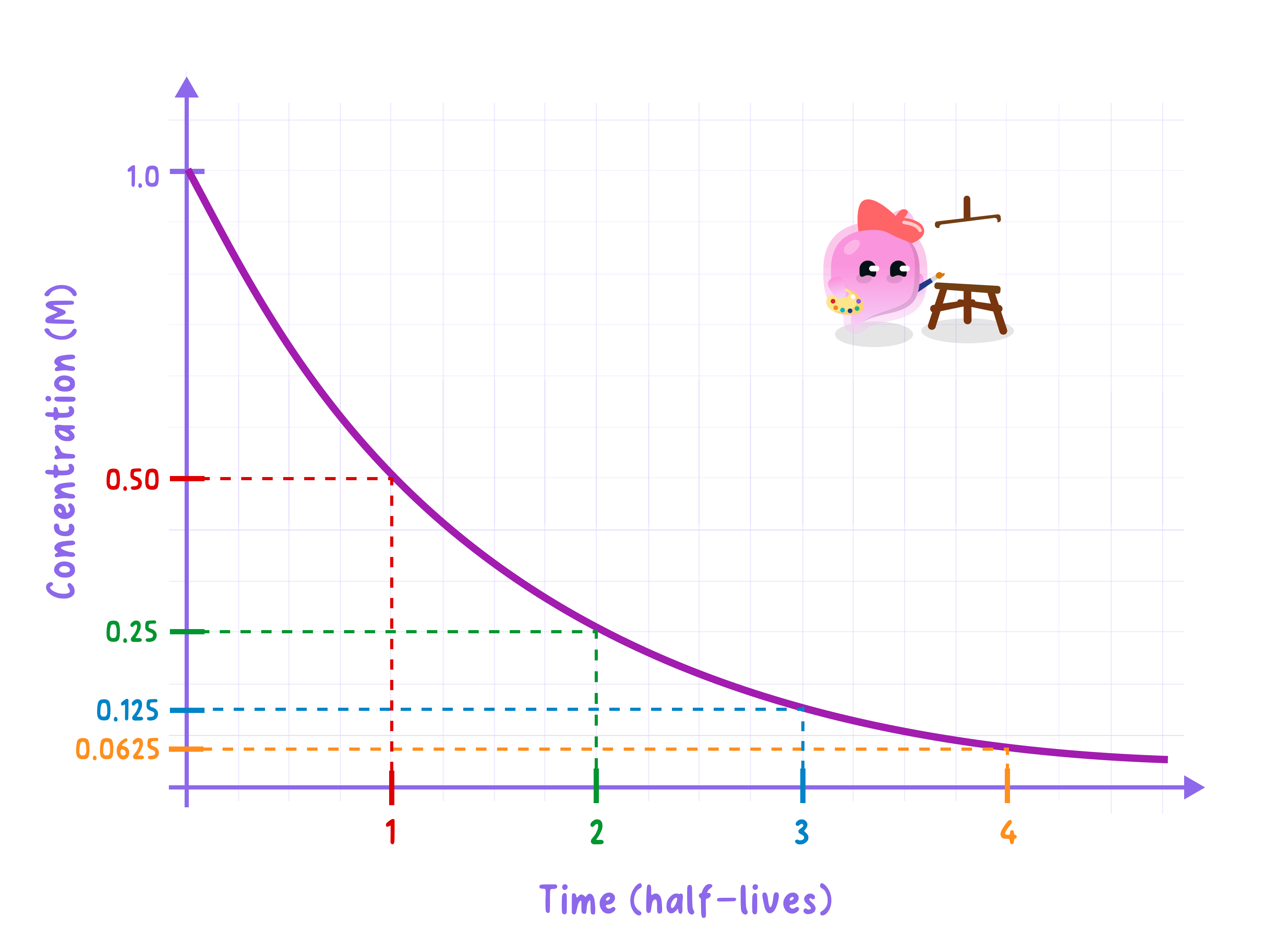
- The defining property is that the same interval of time removes the same fraction of what is left, wherever on the curve you begin.
- So the time to fall from the full amount to a half is the same as the time to fall from a half to a quarter, and the same again from a quarter to an eighth.
- This is why the fall is described as exponential: the step down is always proportional to the amount currently present.
- It also explains the shape of the graph, which is steep at the start where there is most left to lose and shallow later where there is least.
- Because the fraction lost is fixed, the amount remaining never reaches zero on the graph, and the curve approaches the time axis without meeting it.
- A practical consequence is that half-life can be measured from any convenient pair of points on a curve, not only from the starting value, and several such measurements should agree.
Why decay is random
Definition
Random process
A random process is one in which the outcome of any individual event cannot be predicted, so it is impossible to say when a particular nucleus will decay.
- Nothing inside a nucleus counts down to its decay, and a nucleus does not age, wear out or become more likely to decay the longer it has already survived.
- Every undecayed nucleus of a given isotope simply carries the same fixed chance of decaying in the next second.
- It is therefore impossible to predict when a particular nucleus will decay, and impossible to say which nucleus in a sample will be next.
- It is equally impossible to make a chosen nucleus decay sooner or later, because nothing done to the material changes that fixed chance.
- What can be predicted is the behaviour of a very large number of nuclei taken together, and this is exactly what half-life does.
- Even a very small sample holds nuclei in numbers of the order of 102010^{20}1020, so although each one is unpredictable, the fraction that decays in a given interval is almost exactly the same every time.
- Half-life is therefore a statistical quantity: it predicts the activity of a large sample reliably while saying nothing whatever about any individual nucleus.
- The randomness is still visible when the numbers involved are small, which is why a count taken over a few seconds jumps about while the same source counted over several minutes gives a steady value.
- Readings taken late in the decay scatter far more than early ones, because by then too few nuclei remain for the averaging to work well.
- The two ideas fit together rather than contradicting each other: the process is random at the level of one nucleus and predictable at the level of a whole sample.
Practical
Modelling random decay with dice
- Aim: to model radioactive decay with dice, showing that a random process with a fixed chance per interval produces a constant half-life.
- Apparatus: 100100100 identical dice, a large shallow tray with raised sides, a results table, graph paper and a calculator.
- Variables: the throw number stands for time and is the independent variable, the number of dice remaining stands for the number of undecayed nuclei and is the dependent variable, and the starting number of dice, the chance of decay per throw and the shaking technique are controlled.
- What each part of the model stands for:
- One die stands for one undecayed nucleus, and one throw of all the dice stands for one interval of time.
- A die landing on a six has decayed and is removed, so every die carries the same chance of 16\dfrac{1}{6}61 of decaying in each interval.
- Which particular die shows a six is unpredictable, which is the feature of real decay the model exists to show.
- Method:
- Record 100100100 as the number remaining at throw 000, before any dice have been removed.
- Place all 100100100 dice in the tray, shake it so that every die tumbles freely, then tip them out onto a flat surface.
- Remove every die showing a six, count the dice left and record that number against throw 111.
- Return only the remaining dice to the tray, so each throw starts from a smaller population than the one before.
- Repeat for at least 151515 throws, or until fewer than five dice remain, recording the number remaining after every throw.
- Pool the whole class's results by adding the numbers remaining at each throw number, because a larger starting population smooths out the scatter.
- Results: the number remaining falls by roughly the same fraction at each throw, so many dice are removed early and only a few at each of the later throws.
- Processing: plot the number of dice remaining on the vertical axis against throw number on the horizontal axis, draw a smooth curve of best fit rather than joining the points, then check that the number of throws taken to fall from 100100100 to 505050, from 505050 to 252525 and from 252525 to about 121212 come out the same.
- Expected pattern: with a chance of 16\dfrac{1}{6}61 per throw the model gives a half-life of roughly four throws, and the same value is obtained from any part of the curve.
- Watch out: returning removed dice destroys the model, because a decayed nucleus does not come back; one group's data is very noisy near the end and should be pooled; failing to shake the tray properly makes the throws less than random.
- Limitations of the model: a die that survives is completely unchanged, whereas a real decay leaves a new nucleus behind, and real decay runs continuously rather than in separate throws.
- Safety: use a tray with raised sides so that dice are not scattered onto the floor and do not become a trip hazard.
Example
What randomness looks like in a measurement
- A long-lived source is placed a fixed distance from a detector and five successive counts are taken, each lasting 10 s10\ \text{s}10 s.
- The five counts come out noticeably different from one another, even though nothing about the source or the apparatus has changed.
- The variation is not a fault in the equipment; it happens because the number of nuclei that happen to decay in any 10 s10\ \text{s}10 s window is a matter of chance.
- Counting instead for a single interval of 600 s600\ \text{s}600 s gathers so many more decays that the same chance variation becomes a much smaller share of the total.
- The steadier value from the longer count is the reason a radioactivity experiment uses long counting intervals and averages several repeats.
Example
Why pooling the dice results helps
- One group starting with 100100100 dice expects about 171717 sixes on the first throw, but may well remove 111111 or 232323 instead.
- By the twelfth throw only a handful of dice are left, so removing one die or none changes the plotted point a great deal and the curve looks ragged.
- Adding the results of thirty groups makes the population at every throw about thirty times larger.
- The chance variation in each group partly cancels against the others, so the pooled totals sit much closer to the smooth curve.
- The same reasoning applies to a real source: the enormous number of nuclei present is what makes its decay curve smooth.
Exam technique
Stating half-life and randomness
- Define half-life using the words half the undecayed nuclei or half the activity, because a loose statement about the source halving is not precise enough.
- Include the word time in the definition, since half-life is an interval of time.
- When asked about randomness, give both halves: an individual nucleus cannot be predicted, and a large number of nuclei can be.
- Use the phrase cannot be predicted rather than saying decay is unknown or uncertain.
- Justify repeat readings by naming the random nature of decay and the need to average, because reliability and consistency are credited here while accuracy is not.
- For a question on the dice model, link each rule to the thing it represents, since the marks are for the comparison rather than for the procedure.
- If asked why the model is limited, name a specific difference such as the discrete throws, rather than saying only that it is not realistic.
Common Mistake
- Do not define half-life as the time for a source to decay completely, because the activity approaches zero without ever reaching it.
- Do not define half-life as the time for half the mass of the sample to disappear, because the atoms are still there as a different element.
- Do not say that half-life gets shorter as the source decays, because it is constant and applies from any point on the curve.
- Do not claim that half-life can be changed by anything done to the material, because nothing alters the chance of a nucleus decaying.
- Do not take randomness to mean the overall pattern is unpredictable, because a large sample behaves very predictably.
- Do not say a nucleus becomes more likely to decay the longer it has survived, because its chance in the next second never changes.
Self review
- Give two equivalent definitions of half-life.
- Explain why the time to fall from a half to a quarter equals the time to fall from the full amount to a half.
- Why is it impossible to predict when a particular nucleus will decay?
- Why can the activity of a large sample still be predicted?
- Name two things that cannot change the half-life of an isotope.
- In the dice model, what does removing a die showing a six represent?
- State one way in which the dice model differs from real radioactive decay.
