Revision notes for Edexcel AS Level Maths Histograms. Open the guide for explanations and worked examples. Written against the Edexcel AS Level Maths (8MA0) specification, so the content matches what's examinable rather than general Maths background.
Histograms
What you'll learn
- How to handle grouped data measured to the nearest whole number.
- How to calculate and use frequency density.
- How to complete histograms and frequency tables.
- How to estimate probabilities from histogram areas.
Why histograms are needed
A histogram is used for grouped numerical data, especially when the class intervals have different widths.
Unlike a bar chart, the height of a histogram bar is not usually the frequency. In a histogram, the area of each bar represents the frequency.
Definition
Key histogram terms
- A class interval is a group such as 10–14 or 15–18.
- The frequency is the number of observations in a class.
- The class width is the length of the interval on the horizontal axis.
- The frequency density is the height of the bar in a histogram.
Key Idea
The big idea
In a histogram:
frequency=class width×frequency density\text{frequency} = \text{class width} \times \text{frequency density}frequency=class width×frequency densitySo:
frequency density=frequencyclass width\text{frequency density} = \frac{\text{frequency}}{\text{class width}}frequency density=class widthfrequency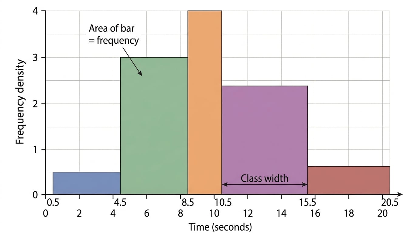
Class widths for rounded data
Many questions say that a variable was measured to the nearest whole number, nearest second, or nearest mile.
This matters because the class 9–13 does not have width 13 − 9 = 4. It contains the whole-number values 9, 10, 11, 12 and 13, so its class width is 5.
Another way to see this is by using class boundaries. If values are measured to the nearest whole number, then the class 9–13 really covers values from 8.5 up to 13.5.
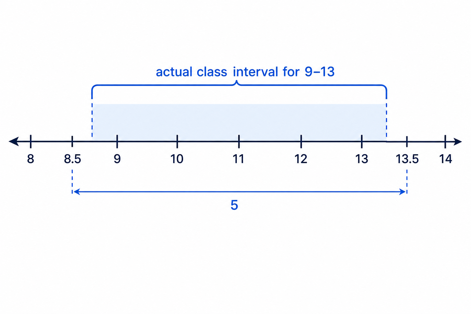
So the width is:
13.5−8.5=513.5 - 8.5 = 513.5−8.5=5Common Mistake
Subtracting the endpoints
For data measured to the nearest whole number, the class 14–20 has width 7, not 6. Count the possible whole-number values, or use boundaries 13.5 to 20.5.
Example
Finding class widths
A variable is measured to the nearest whole number. The grouped classes are 4–8, 9–12, 13–19 and 20–22. Find the class width of each interval.
-
For 4–8, the possible whole-number values are 4, 5, 6, 7 and 8, so the class width is 5.
-
For 9–12, the possible whole-number values are 9, 10, 11 and 12, so the class width is 4.
-
For 13–19, the possible whole-number values are 13, 14, 15, 16, 17, 18 and 19, so the class width is 7.
-
For 20–22, the possible whole-number values are 20, 21 and 22, so the class width is 3.
Calculating frequency density
Once you know the class width, you can calculate the frequency density.
The frequency density tells you how “packed” the frequency is over that interval. A narrow class with a high frequency will have a tall bar. A wide class with the same frequency will have a shorter bar.
Example
Completing a frequency-density table
The times taken to complete a task, measured to the nearest second, are summarised below.
| Time (s) | Frequency |
|---|---|
| 1–3 | 6 |
| 4–7 | 16 |
| 8–10 | 9 |
| 11–15 | missing |
| 16–20 | 5 |
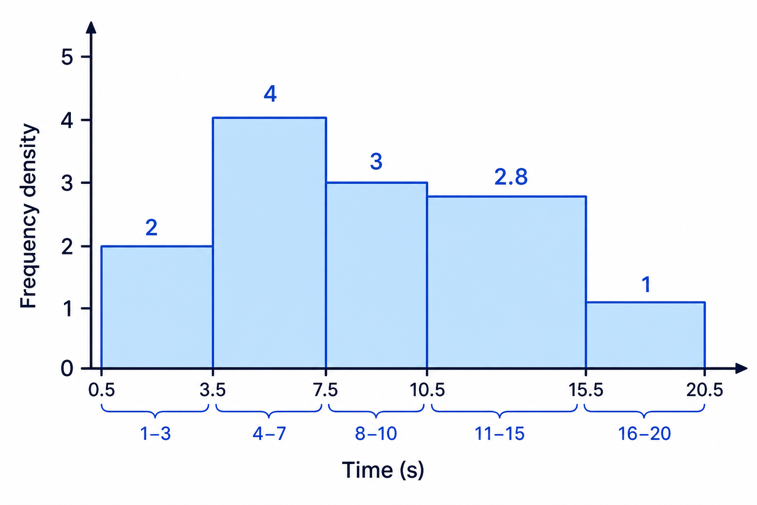
In the histogram, the bar for 11–15 has frequency density 2.8. Find the missing frequency and the frequency density for each class.
-
First find the class widths. Since the times are measured to the nearest second, count the whole-number values in each class: 1–3 has width 3, 4–7 has width 4, 8–10 has width 3, 11–15 has width 5, and 16–20 has width 5.
-
Use the given density for 11–15 to find the missing frequency:
frequency=5×2.8=14\text{frequency} = 5 \times 2.8 = 14frequency=5×2.8=14 -
Now calculate the other frequency densities using frequency density=frequencyclass width\text{frequency density} = \frac{\text{frequency}}{\text{class width}}frequency density=class widthfrequency.
1–3:63=24–7:164=48–10:93=311–15:145=2.816–20:55=1\begin{aligned} 1\text{–}3 &: \frac{6}{3} = 2 \\ 4\text{–}7 &: \frac{16}{4} = 4 \\ 8\text{–}10 &: \frac{9}{3} = 3 \\ 11\text{–}15 &: \frac{14}{5} = 2.8 \\ 16\text{–}20 &: \frac{5}{5} = 1 \end{aligned}1–34–78–1011–1516–20:36=2:416=4:39=3:514=2.8:55=1 -
The completed histogram would have bars with heights 2, 4, 3, 2.8 and 1 respectively.
Tip
Quick check
If two classes have the same frequency but one class is wider, the wider class must have a smaller frequency density.
Drawing or completing a histogram
To draw a histogram:
- Put the variable on the horizontal axis.
- Use class boundaries or consistent class widths.
- Put frequency density on the vertical axis.
- Draw bars so that they touch.
- Make sure each bar’s area represents its frequency.
The bars touch because the data are continuous or being treated as continuous. For example, time, distance and mass can take any value within an interval.
Example
Choosing bar heights for a histogram
A set of distances, measured to the nearest mile, is summarised below.
| Distance (miles) | Frequency |
|---|---|
| 0–4 | 10 |
| 5–9 | 15 |
| 10–14 | 20 |
| 15–19 | 8 |
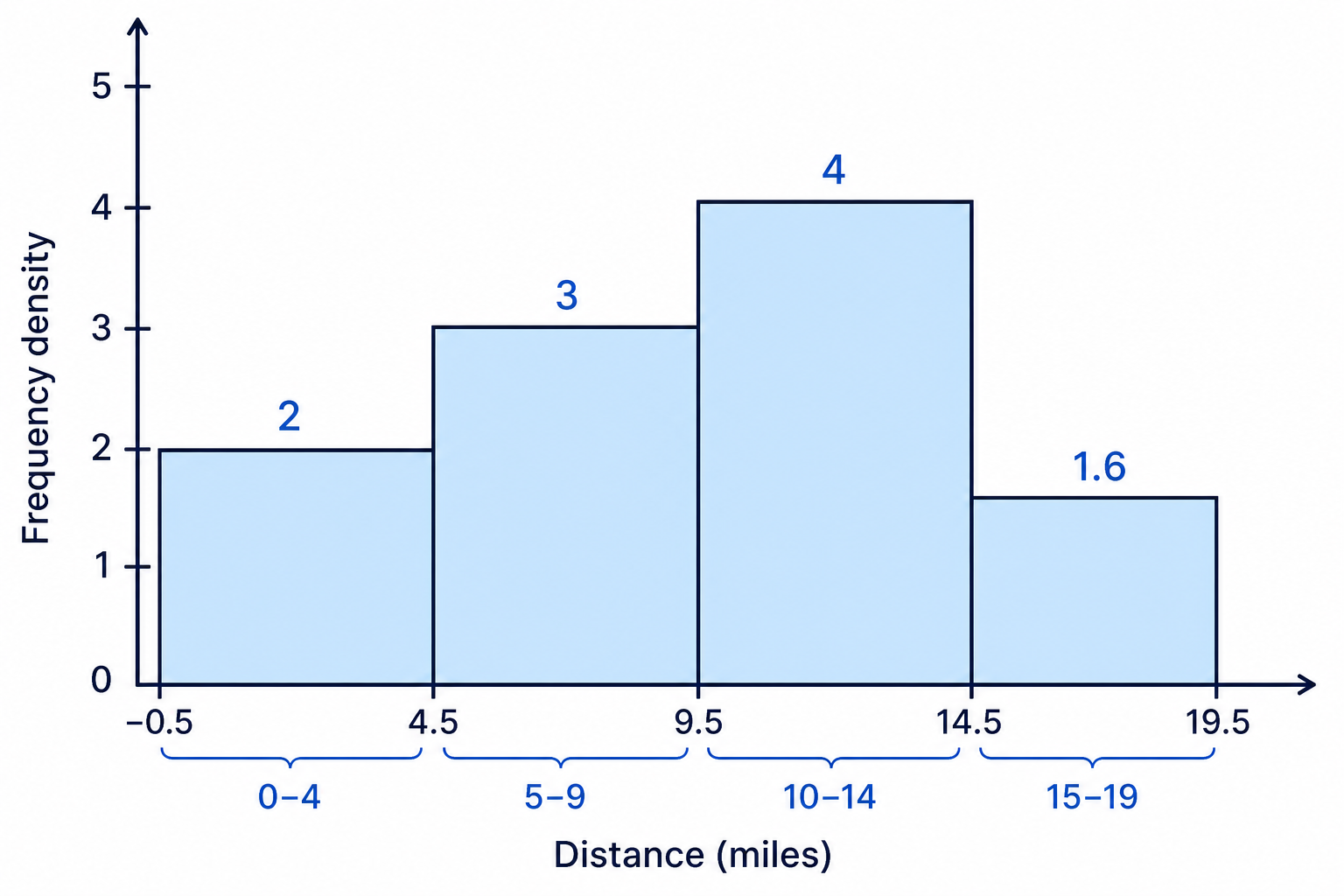
Find the frequency density for each class, ready to draw a histogram.
-
Each class has width 5 because each contains five possible whole-number distances.
-
Divide each frequency by 5.
0–4:105=25–9:155=310–14:205=415–19:85=1.6\begin{aligned} 0\text{–}4 &: \frac{10}{5} = 2 \\ 5\text{–}9 &: \frac{15}{5} = 3 \\ 10\text{–}14 &: \frac{20}{5} = 4 \\ 15\text{–}19 &: \frac{8}{5} = 1.6 \end{aligned}0–45–910–1415–19:510=2:515=3:520=4:58=1.6 -
The histogram bars should therefore have heights 2, 3, 4 and 1.6.
Finding drawn widths and heights from a reference bar
Sometimes you are told the actual size of one bar on the page, for example:
- the bar for 9–13 has width 2 cm;
- the bar for 9–13 has height 2.7 cm.
You then have to find the width and height of another bar.
There are two separate scales:
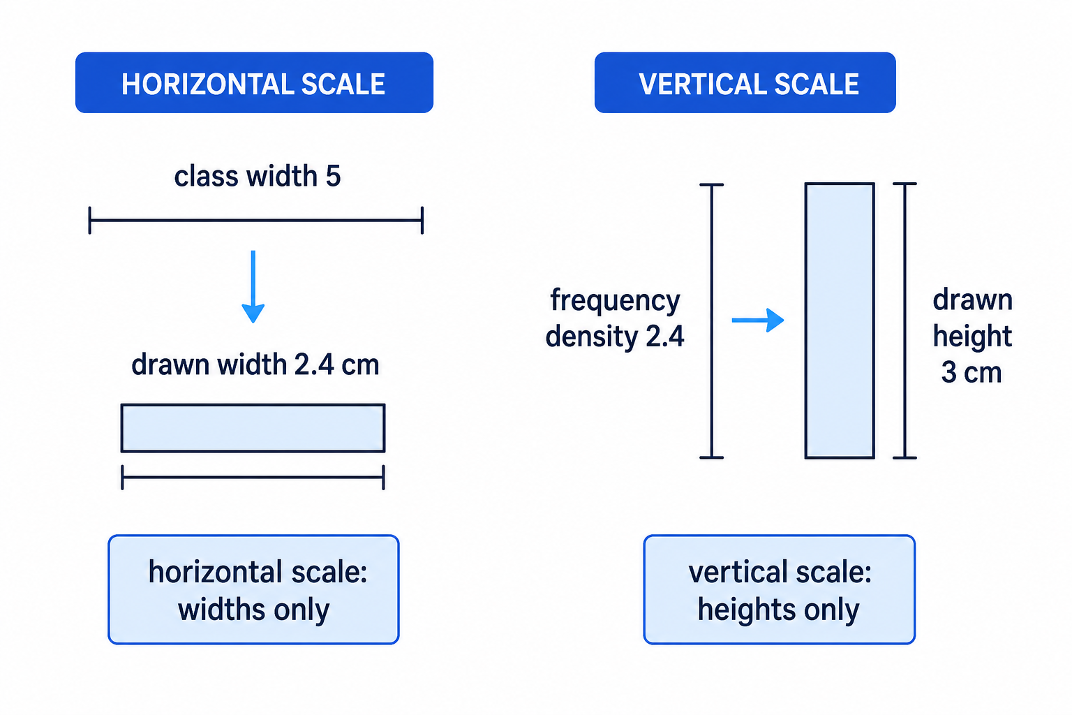
- the horizontal scale, which links class width to drawn width;
- the vertical scale, which links frequency density to drawn height.
Example
Using one bar to find another bar
A variable is measured to the nearest whole number. The table shows some grouped data.
| Class | Frequency |
|---|---|
| 4–8 | 10 |
| 9–13 | 12 |
| 14–20 | 21 |
| 21–24 | 8 |
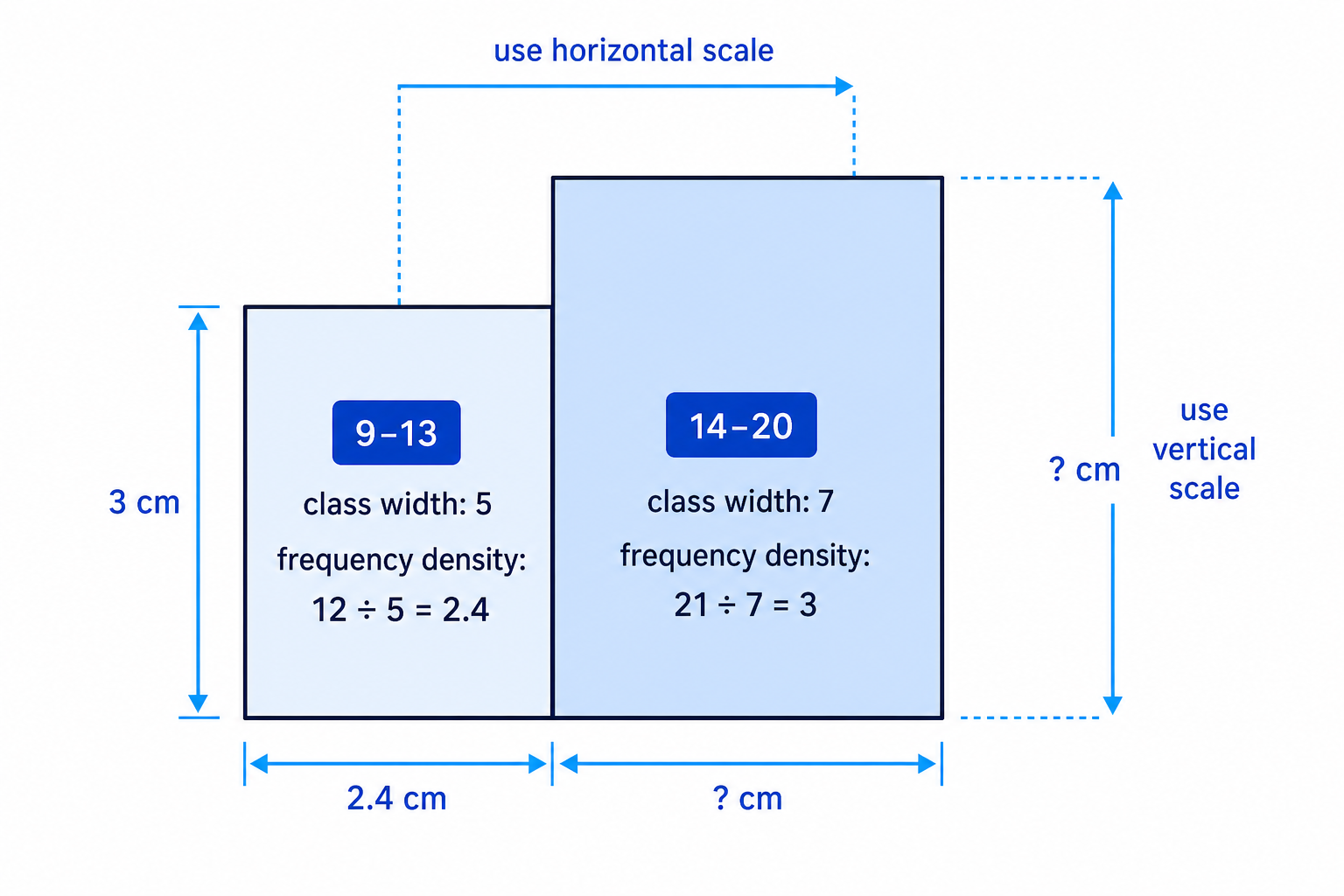
In a histogram, the bar for 9–13 has width 2.4 cm and height 3 cm. Find the width and height of the bar for 14–20.
-
Find the actual class width of the reference class 9–13. It has width 5.
-
Use the reference bar to find the horizontal scale:
2.45=0.48\frac{2.4}{5} = 0.4852.4=0.48 -
The class 14–20 has width 7, so its drawn width is 3.36 cm:
7×0.48=3.367 \times 0.48 = 3.367×0.48=3.36 -
Now find the frequency density of the reference class 9–13:
125=2.4\frac{12}{5} = 2.4512=2.4 -
Since frequency density 2.4 is drawn with height 3 cm, find the vertical scale:
32.4=1.25\frac{3}{2.4} = 1.252.43=1.25 -
The frequency density of the class 14–20 is 3:
217=3\frac{21}{7} = 3721=3 -
Therefore the drawn height of the 14–20 bar is 3.75 cm:
3×1.25=3.753 \times 1.25 = 3.753×1.25=3.75
Common Mistake
Mixing up the two scales
Do not use the width scale to find heights. Widths come from class widths; heights come from frequency densities.
Estimating probabilities from a histogram
If one observation is chosen at random, a probability can be estimated using frequencies.
Since histogram area represents frequency, you can also use areas.
The basic idea is:
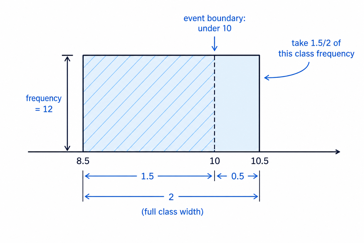
P(event)=estimated frequency for eventtotal frequencyP(\text{event}) = \frac{\text{estimated frequency for event}}{\text{total frequency}}P(event)=total frequencyestimated frequency for eventSometimes the boundary for the event cuts through a class. In that case, assume the data are evenly spread within that class and take the matching fraction of the class frequency.
Example
Estimating a probability using part of a class
The times taken to finish a puzzle, measured to the nearest second, are grouped below.
| Time (s) | Frequency |
|---|---|
| 1–4 | 4 |
| 5–8 | 20 |
| 9–10 | 12 |
| 11–15 | 15 |
| 16–20 | 9 |
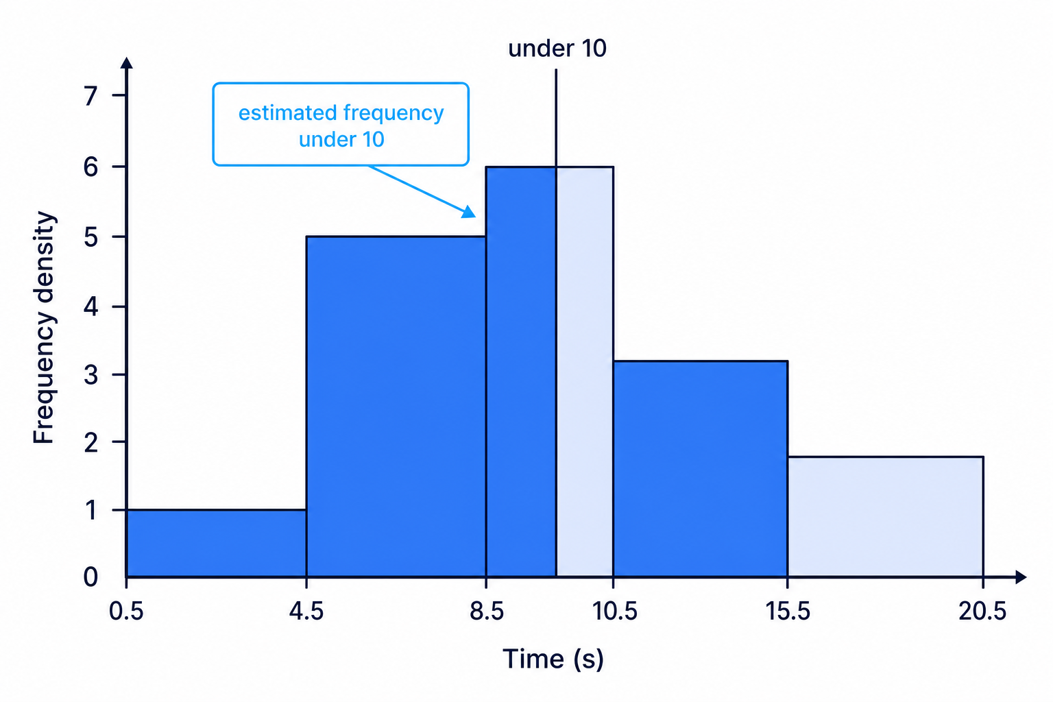
Estimate the probability that a randomly chosen person finished in under 10 seconds.
-
First find the total frequency:
4+20+12+15+9=604 + 20 + 12 + 15 + 9 = 604+20+12+15+9=60 -
The classes 1–4 and 5–8 are completely under 10 seconds, so include their full frequencies:
4+20=244 + 20 = 244+20=24 -
The class 9–10 has boundaries 8.5 to 10.5, so its width is 2. The part under 10 runs from 8.5 to 10, which has width 1.5.
-
Estimate the frequency from the 9–10 class that is under 10 seconds:
1.52×12=9\frac{1.5}{2} \times 12 = 921.5×12=9 -
The estimated number under 10 seconds is 33:
24+9=3324 + 9 = 3324+9=33 -
Therefore the estimated probability is:
P(under 10)=3360=0.55P(\text{under }10) = \frac{33}{60} = 0.55P(under 10)=6033=0.55
Common Mistake
When a boundary cuts through a class
The probability is only an estimate because you do not know exactly how the values are spread inside that class.
Exam technique
In the exam
- Always find the class widths first, especially when values are measured to the nearest whole number.
- Use frequency density, not frequency, for histogram heights.
- If a question gives you one drawn bar in cm, find the horizontal and vertical scales separately.
- For probabilities, use areas or estimated frequencies, and take only the correct fraction of any cut-through class.
Self review
Check yourself
- Why does the class 14–20 have width 7 when data are measured to the nearest whole number?
- What does the area of a histogram bar represent?
- If a class has frequency 18 and width 6, what is its frequency density?

Recap questions
Test yourself with 5 quick questions on this guide. Answer them all correctly to complete it.
You've reached the end
Test yourself on this topic, or move on to the next guide.
How was this guide?