

What you'll learn
- How a sample mean changes when a different random sample is selected.
- Why the sample mean X‾\overline{X}X can itself be treated as a random variable.
- How to find the mean and variance of X‾\overline{X}X.
- How this idea supports statistical hypothesis testing.
From a population to a sample
A population is the complete set of individuals or observations that you want to investigate. A sample is a smaller collection selected from that population.
Suppose a population measurement is represented by the random variable XXX, with:
E(X)=μandVar(X)=σ2.\operatorname{E}(X)=\mu \qquad\text{and}\qquad \operatorname{Var}(X)=\sigma^2.E(X)=μandVar(X)=σ2.Here, μ\muμ is the population mean and σ2\sigma^2σ2 is the population variance.
If you take a random sample of size nnn, its observations can be represented by the random variables
X1,X2,…,Xn.X_1,X_2,\ldots,X_n.X1,X2,…,Xn.Unless the context says otherwise, these observations are normally assumed to be independent and to have the same distribution as XXX.
Independent observations
Observations are independent when knowing the value of one observation does not give you information about the values of the others.
The sample mean
The sample mean is found by adding all the observations in a sample and dividing by the sample size.
Sample mean
For a random sample X1,X2,…,XnX_1,X_2,\ldots,X_nX1,X2,…,Xn, the sample mean is
X‾=X1+X2+⋯+Xnn=1n∑i=1nXi.\overline{X}=\frac{X_1+X_2+\cdots+X_n}{n} =\frac{1}{n}\sum_{i=1}^{n}X_i.X=nX1+X2+⋯+Xn=n1i=1∑nXi.If you have already collected a particular sample, its observed mean is often written using lower-case notation, x‾\overline{x}x.
For example, if the observed sample is 4, 7, 8 and 9, then
x‾=4+7+8+94=7.\overline{x}=\frac{4+7+8+9}{4}=7.x=44+7+8+9=7.The value 7 is fixed once that particular sample has been observed. Before selecting the sample, however, you do not know which observations you will obtain.
Why the sample mean is random
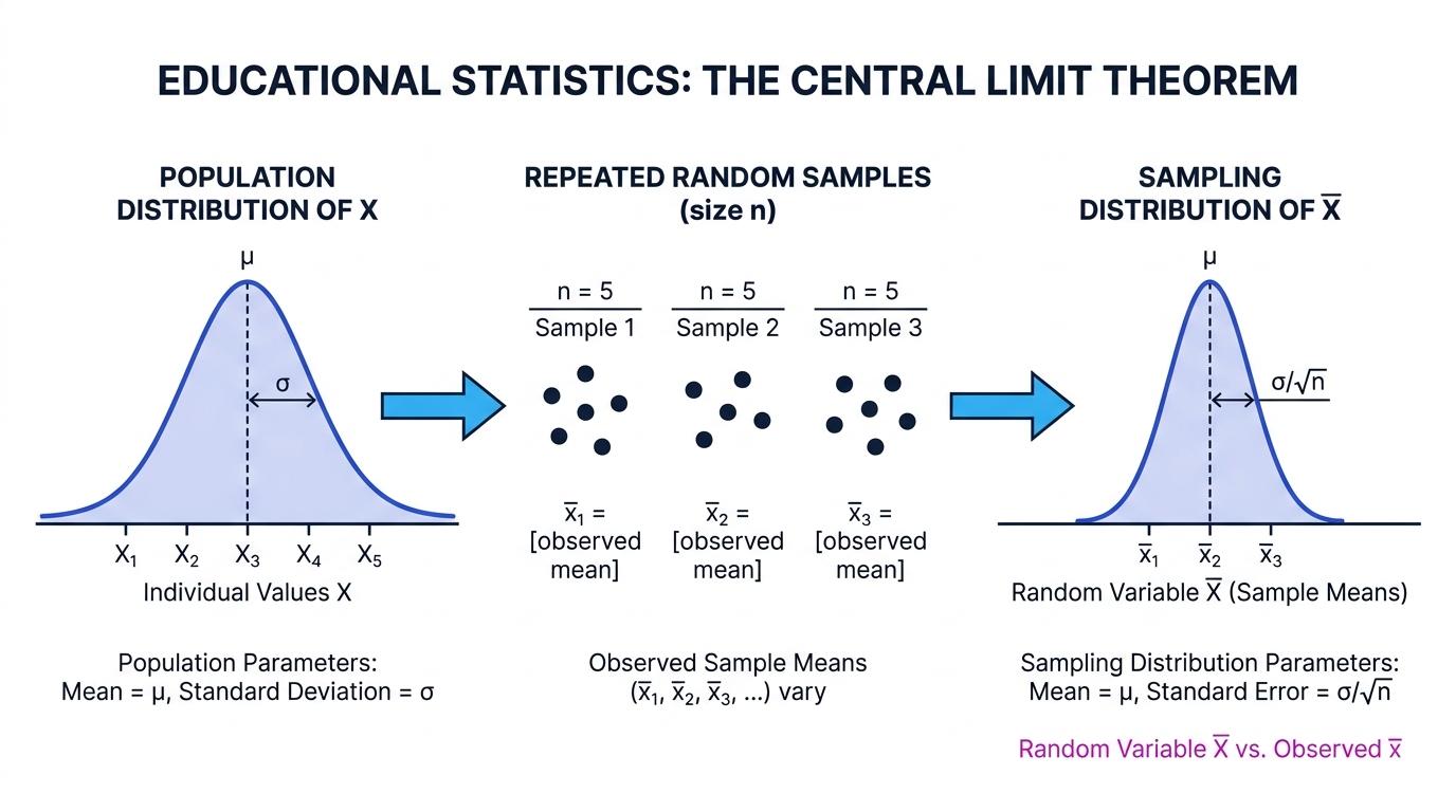
Imagine repeatedly taking random samples of the same size from a population. Different samples will usually contain different observations, so they will usually have different sample means.
Therefore, before a sample is selected, its mean is not a known fixed number. It has a range of possible values, each with an associated probability. This means that X‾\overline{X}X is a random variable.
Sample mean as a random variable
X‾\overline{X}X is the random variable whose value is the mean of a randomly selected sample of size nnn. Its probability distribution is called the sampling distribution of the sample mean.
What is random?
The formula for the mean does not change. The value of the mean is random because the observations included in the sample are random.
Finding the possible sample means
A population consists of the values 2, 4 and 6. Two values are selected independently with replacement.
-
There are nine equally likely ordered samples:
(2,2),(2,4),(2,6),(4,2),(4,4),(4,6),(6,2),(6,4),(6,6).(2,2),(2,4),(2,6),(4,2),(4,4),(4,6),(6,2),(6,4),(6,6).(2,2),(2,4),(2,6),(4,2),(4,4),(4,6),(6,2),(6,4),(6,6). -
Calculating the mean of each sample gives the possible values 2, 3, 4, 5 and 6. For example,
2+42=3and4+62=5.\frac{2+4}{2}=3 \qquad\text{and}\qquad \frac{4+6}{2}=5.22+4=3and24+6=5. -
Counting how often each mean occurs gives
P(X‾=2)=19,P(X‾=3)=29,P(X‾=4)=39,P(X‾=5)=29,P(X‾=6)=19.\begin{aligned} \operatorname{P}(\overline{X}=2)&=\frac{1}{9},\\ \operatorname{P}(\overline{X}=3)&=\frac{2}{9},\\ \operatorname{P}(\overline{X}=4)&=\frac{3}{9},\\ \operatorname{P}(\overline{X}=5)&=\frac{2}{9},\\ \operatorname{P}(\overline{X}=6)&=\frac{1}{9}. \end{aligned}P(X=2)P(X=3)P(X=4)P(X=5)P(X=6)=91,=92,=93,=92,=91. -
These probabilities form the sampling distribution of X‾\overline{X}X. A single selected sample produces one observed value, but X‾\overline{X}X describes all the possible sample means before selection.
The expected value of the sample mean
The expected value of X‾\overline{X}X is the population mean:
E(X‾)=μ.\operatorname{E}(\overline{X})=\mu.E(X)=μ.To see why, use the linearity of expectation:
E(X‾)=E(X1+⋯+Xnn)=1n(E(X1)+⋯+E(Xn))=1n(nμ)=μ.\begin{aligned} \operatorname{E}(\overline{X}) &=\operatorname{E}\left(\frac{X_1+\cdots+X_n}{n}\right)\\ &=\frac{1}{n}\left(\operatorname{E}(X_1)+\cdots+\operatorname{E}(X_n)\right)\\ &=\frac{1}{n}(n\mu)\\ &=\mu. \end{aligned}E(X)=E(nX1+⋯+Xn)=n1(E(X1)+⋯+E(Xn))=n1(nμ)=μ.This makes the sample mean an unbiased estimator of the population mean.
Unbiased estimator
An estimator is unbiased when its expected value equals the population parameter being estimated. Since E(X‾)=μ\operatorname{E}(\overline{X})=\muE(X)=μ, the sample mean is an unbiased estimator of μ\muμ.
Being unbiased does not mean every sample mean equals μ\muμ. It means that, over many repeated samples, the sample means are centred on μ\muμ.
The variance of the sample mean
For independent observations, variances add. Therefore,
Var(X‾)=Var(X1+⋯+Xnn)=1n2(Var(X1)+⋯+Var(Xn))=1n2(nσ2)=σ2n.\begin{aligned} \operatorname{Var}(\overline{X}) &=\operatorname{Var}\left(\frac{X_1+\cdots+X_n}{n}\right)\\ &=\frac{1}{n^2}\left(\operatorname{Var}(X_1)+\cdots+\operatorname{Var}(X_n)\right)\\ &=\frac{1}{n^2}(n\sigma^2)\\ &=\frac{\sigma^2}{n}. \end{aligned}Var(X)=Var(nX1+⋯+Xn)=n21(Var(X1)+⋯+Var(Xn))=n21(nσ2)=nσ2.The standard deviation of X‾\overline{X}X is therefore
Var(X‾)=σn.\sqrt{\operatorname{Var}(\overline{X})} =\frac{\sigma}{\sqrt{n}}.Var(X)=nσ.This standard deviation is called the standard error of the sample mean.
Effect of sample size
As the sample size increases, the sampling distribution becomes less spread out. Larger samples tend to produce means closer to the population mean.
Comparing the spread of sample means
A population has mean μ=50\mu=50μ=50 and standard deviation σ=12\sigma=12σ=12. Consider independent random samples of sizes 9 and 36.
-
For samples with n=9n=9n=9, the standard error is
σn=129=4.\frac{\sigma}{\sqrt{n}} =\frac{12}{\sqrt{9}} =4.nσ=912=4. -
For samples with n=36n=36n=36, the standard error is
1236=2.\frac{12}{\sqrt{36}} =2.3612=2. -
Both sampling distributions have expected value 50, but the means from samples of size 36 are less variable. Multiplying the sample size by 4 has divided the standard error by 2.
Dividing the variance incorrectly
The variance is σ2n\frac{\sigma^2}{n}nσ2, while the standard deviation is σn\frac{\sigma}{\sqrt{n}}nσ. Do not use σn\frac{\sigma}{n}nσ as the standard deviation.
Independence matters
The calculation Var(X‾)=σ2n\operatorname{Var}(\overline{X})=\frac{\sigma^2}{n}Var(X)=nσ2 assumes independent observations with common variance σ2\sigma^2σ2. Sampling without replacement from a small finite population can make the observations dependent.
Connection to hypothesis testing
In a hypothesis test about a population mean, the null hypothesis proposes a value for μ\muμ. You then consider how the random variable X‾\overline{X}X should behave if that proposed value is correct.
An observed sample gives a particular value x‾\overline{x}x. If this value lies unusually far into a tail of the sampling distribution predicted by the null hypothesis, it provides evidence against the null hypothesis.
Keep the notation distinct
Use X‾\overline{X}X for the random variable representing all possible sample means, and x‾\overline{x}x for the numerical mean obtained from the sample actually observed.
In the exam
- State that X‾\overline{X}X is random because different random samples can produce different sample means.
- Use E(X‾)=μ\operatorname{E}(\overline{X})=\muE(X)=μ and, for independent observations, Var(X‾)=σ2n\operatorname{Var}(\overline{X})=\frac{\sigma^2}{n}Var(X)=nσ2.
- Check whether the question asks for variance or standard deviation: the standard deviation is σn\frac{\sigma}{\sqrt{n}}nσ.
- Distinguish the random variable X‾\overline{X}X from an observed value x‾\overline{x}x.
Check yourself
- Why can X‾\overline{X}X be a random variable even though it is calculated using a fixed formula?
- A population has standard deviation 15. What is the standard error of the mean for samples of size 25?
- What happens to the expected value and variance of X‾\overline{X}X when the sample size increases?
