

What you'll learn
- How to translate a real-world problem into an equation whose roots have meaning.
- How to choose and apply a suitable numerical method.
- How to interpret, round and check a numerical solution in its original context.
- How to recognise when a mathematical root is not a valid practical answer.
Prerequisites
Before using numerical methods in context, you should be familiar with:
- locating a root using a change of sign;
- interval-search methods such as bisection;
- fixed-point iteration, written xn+1=g(xn)x_{n+1}=g(x_n)xn+1=g(xn);
- the Newton–Raphson method:
In this section, the main challenge is not usually carrying out the iteration. It is deciding what equation to solve and what the resulting value means.
From a context to a root
A mathematical model is a simplified mathematical description of a real situation. The model may involve quantities such as cost, time, distance, temperature or population.
Suppose the context gives two quantities A(x)A(x)A(x) and B(x)B(x)B(x) and asks when they are equal. You begin with
A(x)=B(x).A(x)=B(x).A(x)=B(x).Numerical root-finding methods are normally applied to an equation of the form f(x)=0f(x)=0f(x)=0, so rearrange this as
f(x)=A(x)−B(x)=0.f(x)=A(x)-B(x)=0.f(x)=A(x)−B(x)=0.Root
A root of the equation f(x)=0f(x)=0f(x)=0 is a value of xxx for which the function has value zero. It is also an xxx-coordinate where the graph of y=f(x)y=f(x)y=f(x) crosses or touches the xxx-axis.
For example, a business breaks even when its revenue equals its cost. If the revenue is R(x)R(x)R(x) and the cost is C(x)C(x)C(x), define
f(x)=R(x)−C(x).f(x)=R(x)-C(x).f(x)=R(x)−C(x).A break-even point is then a root of f(x)=0f(x)=0f(x)=0.
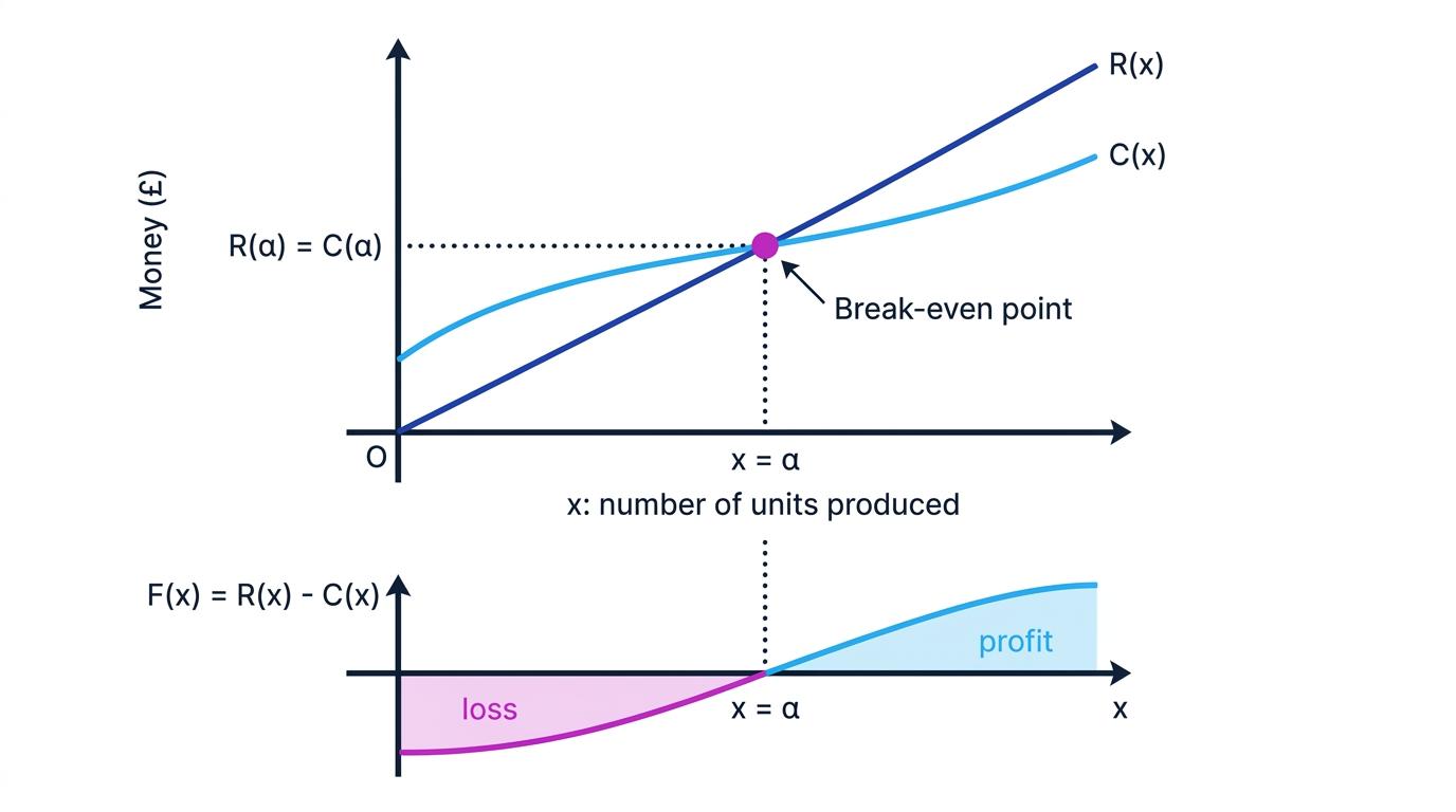
Create a zero equation
Numerical methods solve equations of the form f(x)=0f(x)=0f(x)=0. In context, your first task is therefore to identify the quantities that must be equal and subtract one side from the other.
Restricting the domain
The domain is the set of values that the variable is allowed to take.
A pure equation may have several roots, but the context can restrict which ones are acceptable. For example:
- time normally requires t≥0t\geq 0t≥0;
- a length must be positive;
- a probability must satisfy 0≤p≤10\leq p\leq 10≤p≤1;
- a number of complete items usually has to be an integer;
- a model may only be stated to apply over a particular interval.
Accepting every root
Do not report a root merely because your calculator or iteration produced it. Check its sign, units, domain and practical meaning.
Locating a relevant root
If fff is continuous and f(a)f(a)f(a) and f(b)f(b)f(b) have opposite signs, then there is at least one root between aaa and bbb.
This is written
f(a)f(b)<0.f(a)f(b)<0.f(a)f(b)<0.The conclusion depends on continuity, meaning that the graph has no break or jump over the interval.
Change of sign
A change of sign occurs when one function value is positive and another is negative. For a continuous function, this confirms that the graph crosses the axis somewhere between those inputs.
A change of sign proves that there is at least one crossing root in the interval, but it does not automatically prove that there is exactly one root.
Choosing a numerical method
The question may specify the method. If it does not, consider the information available.
Interval search
Use an interval method such as bisection when you have a change of sign. It is reliable because each stage keeps the root trapped inside a smaller interval.
Fixed-point iteration
If the equation has been rearranged as x=g(x)x=g(x)x=g(x), use
xn+1=g(xn).x_{n+1}=g(x_n).xn+1=g(xn).The sequence must converge, meaning that its terms approach a fixed value. Some rearrangements converge while others diverge, even though they come from the same original equation.
Newton–Raphson
If f′(x)f'(x)f′(x) is available and you have a suitable starting value, Newton–Raphson often converges quickly:
xn+1=xn−f(xn)f′(xn).x_{n+1}=x_n-\frac{f(x_n)}{f'(x_n)}.xn+1=xn−f′(xn)f(xn).It can fail or move towards an unintended root if the starting value is poor or if f′(xn)f'(x_n)f′(xn) is zero or very small.
Use the context to choose a starting value
A graph, a given interval or an earlier estimate should guide your starting value. Do not choose it without considering which root the context requires.
A complete contextual problem
A company produces xxx items each day. Its cost and revenue, in pounds, are modelled by
C(x)=500+8xC(x)=500+8xC(x)=500+8xand
R(x)=20x−0.02x2.R(x)=20x-0.02x^2.R(x)=20x−0.02x2.We will find the first production level at which the company makes a profit.
Finding a break-even production level
-
Break-even occurs when revenue equals cost. Define the profit function:
P(x)=R(x)−C(x)=20x−0.02x2−(500+8x)=−0.02x2+12x−500.\begin{aligned} P(x)&=R(x)-C(x)\\ &=20x-0.02x^2-(500+8x)\\ &=-0.02x^2+12x-500. \end{aligned}P(x)=R(x)−C(x)=20x−0.02x2−(500+8x)=−0.02x2+12x−500.We therefore need to solve P(x)=0P(x)=0P(x)=0.
-
Locate the first root by testing nearby production levels:
P(45)=−0.5,P(46)=9.68.\begin{aligned} P(45)&=-0.5,\\ P(46)&=9.68. \end{aligned}P(45)P(46)=−0.5,=9.68.Since the profit function is continuous and changes sign, there is a break-even point in the interval 45<x<4645<x<4645<x<46.
-
Refine the interval:
P(45.04)=−0.092032,P(45.05)=0.00995.\begin{aligned} P(45.04)&=-0.092032,\\ P(45.05)&=0.00995. \end{aligned}P(45.04)P(45.05)=−0.092032,=0.00995.The break-even point is therefore between 45.04 and 45.05 items, approximately x=45.049x=45.049x=45.049.
-
Interpret the result. The company cannot normally produce 45.049 complete items. At 45 items the model gives a loss, while at 46 items it gives a profit. The first whole-number production level giving a profit is therefore 46 items.
This example shows why contextual rounding is different from ordinary decimal rounding. Although the root rounds to 45 to the nearest integer, producing 45 items does not meet the required condition.
Rounding without checking
When the answer counts complete objects, substitute the neighbouring integers into the model. Ordinary rounding may give an integer that does not satisfy the practical requirement.
Checking the approximation
Once an iterative process appears to have converged, substitute the result back into the original equation.
If α\alphaα is your approximate root, calculate f(α)f(\alpha)f(α). A value close to zero supports the approximation, allowing for rounding error.
However, repeated decimal values alone do not prove that you have found the required solution. You must also check:
- whether the value belongs to the permitted domain;
- whether the method has approached the intended root;
- whether the requested accuracy has been achieved;
- whether the answer makes sense in the context.
Checking a numerical root
Suppose Newton–Raphson gives the approximate break-even value x=45.049x=45.049x=45.049.
-
Substitute it into the profit model:
P(45.049)=−0.02(45.049)2+12(45.049)−500.P(45.049)=-0.02(45.049)^2+12(45.049)-500.P(45.049)=−0.02(45.049)2+12(45.049)−500. -
Evaluating gives a result very close to zero, with any small difference caused by using the rounded value 45.04945.04945.049 rather than the full calculator value.
-
Since 45.04945.04945.049 also lies in the previously established interval 45.04<x<45.0545.04<x<45.0545.04<x<45.05, the approximation is consistent with the sign-change check.
Accuracy in context
A question may request a number of decimal places or significant figures. Keep extra calculator digits during the iteration and round only the final result.
Sometimes the context determines the appropriate form instead:
- Money may be given to the nearest penny.
- Time might be required to the nearest second.
- A measurement might be given to a stated number of significant figures.
- A number of people, vehicles or products must usually be a whole number.
Numerical accuracy and practical accuracy
A highly accurate decimal approximation is not automatically a useful final answer. Your reported value must have sensible units and precision for the situation.
Limitations of the model
A numerical method may solve the model accurately even when the model itself is only an approximation.
For example, a cost model may assume that the cost per item remains constant. In reality, discounts, limited capacity or changing wages could make that assumption unreliable.
An accurate root can still model reality poorly
Numerical error and modelling error are different. More iterations reduce numerical error, but they do not improve unrealistic assumptions in the original model.
Writing the conclusion
Finish with a sentence that answers the actual question, including units where appropriate.
For example:
The model predicts that the company must produce at least 46 items per day to make a profit.
Avoid ending with only a calculator value such as x=45.049x=45.049x=45.049, because this does not fully interpret the solution.
In the exam
- Define a function f(x)f(x)f(x) so that the required condition becomes f(x)=0f(x)=0f(x)=0.
- State the relevant interval, domain restriction or starting value before applying the numerical method.
- Keep unrounded values during the calculation, then check and interpret the final approximation using the context.
- Include appropriate units and test neighbouring integers when the quantity must be whole.
Check yourself
- How would you turn an equation A(x)=B(x)A(x)=B(x)A(x)=B(x) into a root-finding problem?
- Why might a mathematically correct negative root need to be rejected?
- If a model gives a minimum required quantity of x=18.2x=18.2x=18.2 objects, how would you decide whether the practical answer is 18 or 19?
