

What you'll learn
- How to recognise exponential growth and exponential decay.
- How to build models using powers or the exponential function.
- How to determine unknown parameters from data.
- How to use and assess predictions made by an exponential model.
Repeated proportional change
An exponential model is appropriate when a quantity changes by the same proportion over equal intervals.
For example, if a population increases by 8% each year, each new population is found by multiplying the previous population by 1.08. The numerical increase is not constant because 8% is being taken of a changing quantity.
This is different from a linear model, in which the same amount is added or subtracted during each interval.
Exponential model
An exponential model has the form
P=P0bt,P=P_0b^t,P=P0bt,where:
- PPP is the quantity after time ttt;
- P0P_0P0 is the initial value, meaning the value when t=0t=0t=0;
- bbb is the constant multiplication factor for one unit of time.
Substituting t=0t=0t=0 gives P=P0b0=P0P=P_0b^0=P_0P=P0b0=P0, confirming that P0P_0P0 is the initial value.
Additive or multiplicative?
- Constant difference over equal intervals suggests a linear model.
- Constant ratio over equal intervals suggests an exponential model.
Recognising exponential change
A culture contains 500 bacteria and increases by 12% each hour. Form a model for the number NNN after ttt hours.
-
An increase of 12% means that 112% of the bacteria remain after each hour, so the multiplication factor is
b=1+12100=1.12.b=1+\frac{12}{100}=1.12.b=1+10012=1.12. -
The initial value is N0=500N_0=500N0=500, because there are 500 bacteria when t=0t=0t=0.
-
Substitute these values into N=N0btN=N_0b^tN=N0bt:
N=500(1.12)t.N=500(1.12)^t.N=500(1.12)t.
Growth and decay
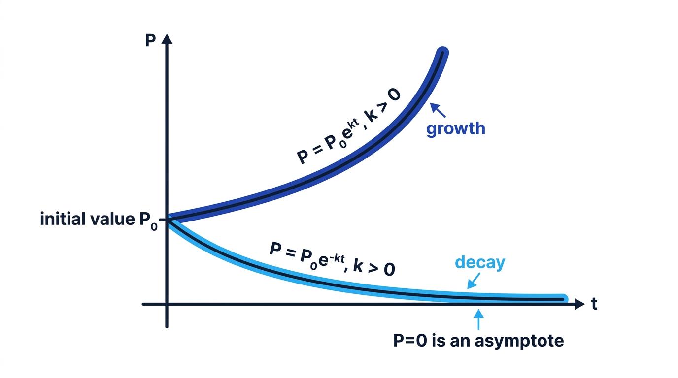
The value of the factor bbb determines whether the model represents growth or decay.
- If b>1b>1b>1, the quantity shows exponential growth.
- If 0<b<10<b<10<b<1, the quantity shows exponential decay.
For growth at a rate of rrr per time interval, written as a decimal,
P=P0(1+r)t.P=P_0(1+r)^t.P=P0(1+r)t.For decay at a rate of rrr per time interval,
P=P0(1−r)t.P=P_0(1-r)^t.P=P0(1−r)t.The growth curve becomes increasingly steep. The decay curve approaches zero but never reaches it according to the mathematical model.
Subtracting a percentage of the initial value
A percentage decrease is normally applied to the current value each time, not repeatedly subtracted from the initial value. This produces multiplicative, rather than linear, change.
Modelling annual depreciation
A machine is initially worth £24,000 and loses 18% of its value each year. Find its model and its value after 5 years.
-
A decrease of 18% leaves 82% of the previous value, so the annual multiplication factor is
b=1−18100=0.82.b=1-\frac{18}{100}=0.82.b=1−10018=0.82. -
Using the initial value £24,000 gives
V=24000(0.82)t.V=24000(0.82)^t.V=24000(0.82)t. -
At t=5t=5t=5,
V=24000(0.82)5≈8897.76.V=24000(0.82)^5\approx8897.76.V=24000(0.82)5≈8897.76.The predicted value after 5 years is approximately £8,898.
Models using the exponential function
Exponential models are also commonly written using the exponential function exe^xex:
P=P0ekt.P=P_0e^{kt}.P=P0ekt.Continuous growth constant
In P=P0ektP=P_0e^{kt}P=P0ekt, the parameter kkk is the continuous growth constant or continuous decay constant.
- If k>0k>0k>0, the model represents growth.
- If k<0k<0k<0, the model represents decay.
- A larger value of ∣k∣\lvert k\rvert∣k∣ means faster change.
The power model and the exponential-function model are equivalent because
bt=(elnb)t=etlnb.b^t=\left(e^{\ln b}\right)^t=e^{t\ln b}.bt=(elnb)t=etlnb.Therefore,
b=ekandk=lnb.b=e^k \qquad\text{and}\qquad k=\ln b.b=ekandk=lnb.The value of kkk depends on the unit used for time. A rate constant measured per day will not have the same numerical value as one measured per hour.
Converting between exponential forms
A quantity is modelled by P=700(1.06)tP=700(1.06)^tP=700(1.06)t. Express the model in the form P=700ektP=700e^{kt}P=700ekt.
-
Compare btb^tbt with ekte^{kt}ekt. Since b=ekb=e^kb=ek, the required constant satisfies
ek=1.06.e^k=1.06.ek=1.06. -
Take natural logarithms:
k=ln(1.06)≈0.05827.k=\ln(1.06)\approx0.05827.k=ln(1.06)≈0.05827. -
The equivalent model is therefore
P=700e0.05827t.P=700e^{0.05827t}.P=700e0.05827t.
Finding a model from two values
Suppose you know that a quantity has value P1P_1P1 at time t1t_1t1 and value P2P_2P2 at time t2t_2t2. For a model P=AektP=Ae^{kt}P=Aekt,
P1=Aekt1andP2=Aekt2.P_1=Ae^{kt_1} \qquad\text{and}\qquad P_2=Ae^{kt_2}.P1=Aekt1andP2=Aekt2.Dividing the equations eliminates AAA:
P2P1=ek(t2−t1).\frac{P_2}{P_1}=e^{k(t_2-t_1)}.P1P2=ek(t2−t1).Taking natural logarithms then gives
k=ln(P2/P1)t2−t1.k=\frac{\ln(P_2/P_1)}{t_2-t_1}.k=t2−t1ln(P2/P1).Once you have found kkk, substitute into either original equation to find AAA.
Determining a population model
A population is 120 at time t=0t=0t=0 and 300 after 8 hours. Model the population by P=AektP=Ae^{kt}P=Aekt, then predict the population after 12 hours.
-
At t=0t=0t=0,
120=Ae0=A,120=Ae^{0}=A,120=Ae0=A,so A=120A=120A=120.
-
Use the value after 8 hours:
300=120e8k.300=120e^{8k}.300=120e8k.Hence
e8k=2.5.e^{8k}=2.5.e8k=2.5. -
Take natural logarithms and solve for kkk:
8k=ln(2.5)⇒k=ln(2.5)8≈0.1145.8k=\ln(2.5) \quad\Rightarrow\quad k=\frac{\ln(2.5)}{8}\approx0.1145.8k=ln(2.5)⇒k=8ln(2.5)≈0.1145. -
The model is
P=120e0.1145t.P=120e^{0.1145t}.P=120e0.1145t.At t=12t=12t=12,
P=120e0.1145(12)≈474.P=120e^{0.1145(12)}\approx474.P=120e0.1145(12)≈474.The model predicts a population of approximately 474.
Keep accuracy during modelling
Keep the exact logarithmic value of kkk, or store the full calculator value. Rounding kkk too early can noticeably change later predictions.
Doubling time and half-life
The doubling time is the time taken for a growing quantity to become twice its current value.
For P=P0ektP=P_0e^{kt}P=P0ekt with k>0k>0k>0, set P=2P0P=2P_0P=2P0:
2P0=P0ekt⇒t=ln2k.2P_0=P_0e^{kt} \quad\Rightarrow\quad t=\frac{\ln 2}{k}.2P0=P0ekt⇒t=kln2.The half-life is the time taken for a decaying quantity to become half its current value. If the model is written as P=P0e−ktP=P_0e^{-kt}P=P0e−kt with k>0k>0k>0, then
t=ln2k.t=\frac{\ln 2}{k}.t=kln2.A decay model with half-life hhh can also be written directly as
P=P0(12)t/h.P=P_0\left(\frac12\right)^{t/h}.P=P0(21)t/h.Using a half-life model
A medicine has an initial mass of 80 mg in the bloodstream and a half-life of 6 hours. Find the mass remaining after 15 hours.
-
The quantity is multiplied by 12\frac1221 every 6 hours, so the model is
M=80(12)t/6.M=80\left(\frac12\right)^{t/6}.M=80(21)t/6. -
Substitute t=15t=15t=15:
M=80(12)15/6.M=80\left(\frac12\right)^{15/6}.M=80(21)15/6. -
Evaluating gives
M≈14.1.M\approx14.1.M≈14.1.Approximately 14.1 mg remains after 15 hours.
Using a model responsibly
A mathematical model is a simplified description of reality. Exponential growth assumes that the same proportional growth rate continues indefinitely, while exponential decay assumes that the same proportional loss continues.
These assumptions may only be reasonable over a limited time interval. For example, a population cannot grow exponentially forever if food, space or other resources are limited.
A prediction made within the range of observed data is called interpolation. A prediction made outside that range is called extrapolation, and it is usually less reliable.
Long-term extrapolation
An exponential formula may produce a numerical answer for any value of ttt, but that does not mean the answer is realistic. State relevant limitations when the context suggests the rate cannot remain constant.
In the exam
- Identify the initial value, the time unit and whether the change is growth or decay.
- Convert a percentage into a multiplier carefully: use 1+r1+r1+r for growth and 1−r1-r1−r for decay.
- When finding parameters, substitute the given data and use logarithms to bring an unknown exponent down.
- Keep full calculator accuracy until the final answer, then round appropriately for the context.
- Check that your prediction is sensible and note when it relies on extrapolation.
Check yourself
- How can you distinguish exponential change from linear change using values at equally spaced times?
- How would you find kkk if a model P=P0ektP=P_0e^{kt}P=P0ekt passes through two known points?
- What assumptions are being made when an exponential population model is used to predict far into the future?
