

What you'll learn
- Recognise and use exponential models in the forms y=abty=ab^ty=abt and y=Aekty=Ae^{kt}y=Aekt.
- Calculate future values, growth rates, decay rates, doubling times and half-lives.
- Use logarithms to find an unknown time.
- Apply exponential models and consider their limitations and possible refinements.
Prerequisites
Before starting, you should be comfortable with:
- index laws, such as aman=am+na^m a^n=a^{m+n}aman=am+n;
- logarithms, especially lnx\ln xlnx, the natural logarithm;
- solving equations by taking logarithms;
- converting a percentage change into a multiplier.
For example, an increase of 6% gives the multiplier 1.061.061.06, while a decrease of 6% gives the multiplier 0.940.940.94.
What is an exponential model?
An exponential model describes a quantity that changes by the same proportion over equal time intervals. This is different from a linear model, where the quantity changes by the same amount.
For example, if a population grows by 4% each year, the number added each year increases as the population itself becomes larger.
Exponential model
A discrete exponential model can be written as
y=abt,y=ab^t,y=abt,where aaa is the initial value, bbb is the multiplier for each time interval, and ttt is the number of time intervals.
- If b>1b>1b>1, the model represents exponential growth.
- If 0<b<10<b<10<b<1, the model represents exponential decay.
- When t=0t=0t=0, b0=1b^0=1b0=1, so y=ay=ay=a. Therefore, aaa is the value at the start.
Modelling annual population growth
A town has an initial population of 24,000 and its population increases by 3.2% each year. Find the predicted population after 8 years.
-
Convert the percentage increase into a multiplier:
b=1+3.2100=1.032.b=1+\frac{3.2}{100}=1.032.b=1+1003.2=1.032. -
Form the model, where ttt is measured in years:
P=24000(1.032)t.P=24000(1.032)^t.P=24000(1.032)t. -
Substitute t=8t=8t=8:
P=24000(1.032)8≈30878.P=24000(1.032)^8\approx30878.P=24000(1.032)8≈30878.The model predicts a population of approximately 30,900 people.
Using the percentage as the multiplier
A growth rate of 3.2% gives a multiplier of 1.0321.0321.032, not 0.0320.0320.032. For decay, subtract the percentage from 100% before forming the multiplier.
Continuous exponential models
At A-level, exponential models are often written using the number eee, where
e≈2.718.e\approx2.718.e≈2.718.The function exe^xex is especially useful because its rate of change is equal to its current value.
Continuous exponential model
A continuous exponential model has the form
Q=Q0ekt,Q=Q_0e^{kt},Q=Q0ekt,where Q0Q_0Q0 is the initial quantity, ttt is time and kkk is the growth constant or decay constant.
The word continuous means that the model allows the quantity to change at every instant, rather than only at the end of fixed intervals.
- If k>0k>0k>0, QQQ grows.
- If k<0k<0k<0, QQQ decays.
- The size of ∣k∣|k|∣k∣ controls how rapidly the quantity changes.
The forms Q=Q0btQ=Q_0b^tQ=Q0bt and Q=Q0ektQ=Q_0e^{kt}Q=Q0ekt are equivalent because
bt=etlnb.b^t=e^{t\ln b}.bt=etlnb.Therefore,
k=lnbandb=ek.k=\ln b \qquad\text{and}\qquad b=e^k.k=lnbandb=ek.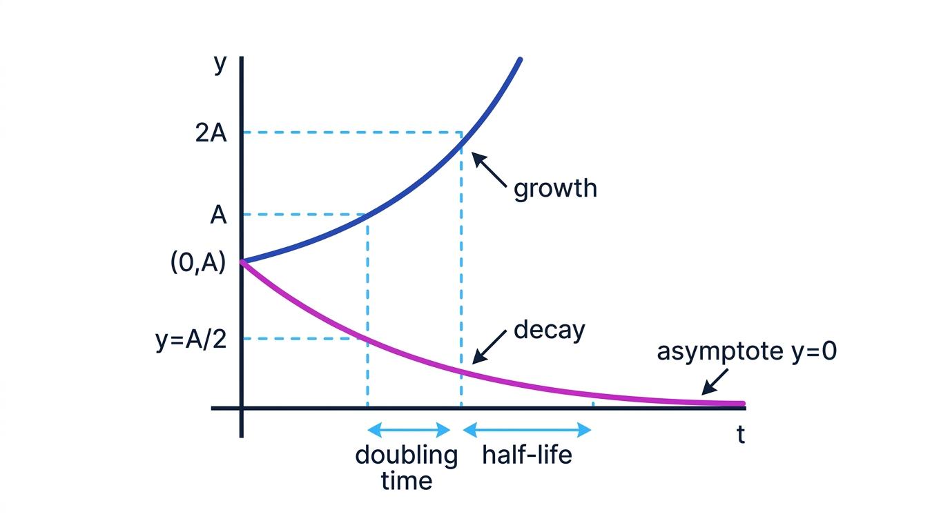
Both curves pass through (0,Q0)(0,Q_0)(0,Q0). A decay curve approaches the horizontal asymptote Q=0Q=0Q=0, but the mathematical model never reaches zero at a finite time.
Converting to an exponential model using e
A population increases by 7% each year. Express its model in the form P=P0ektP=P_0e^{kt}P=P0ekt.
-
The annual multiplier is 1.071.071.07, so
P=P0(1.07)t.P=P_0(1.07)^t.P=P0(1.07)t. -
Use bt=etlnbb^t=e^{t\ln b}bt=etlnb:
(1.07)t=etln(1.07).(1.07)^t=e^{t\ln(1.07)}.(1.07)t=etln(1.07). -
Therefore,
P=P0etln(1.07)≈P0e0.06766t.P=P_0e^{t\ln(1.07)} \approx P_0e^{0.06766t}.P=P0etln(1.07)≈P0e0.06766t.The continuous growth constant is approximately 0.067660.067660.06766 per year.
Finding an unknown time
If the unknown appears in an exponent, use logarithms to bring it down.
For the model
Q=Q0ekt,Q=Q_0e^{kt},Q=Q0ekt,divide by Q0Q_0Q0 and take natural logarithms:
QQ0=ekt\frac{Q}{Q_0}=e^{kt}Q0Q=ekt ln(QQ0)=kt.\ln\left(\frac{Q}{Q_0}\right)=kt.ln(Q0Q)=kt.Hence,
t=ln(Q/Q0)k.t=\frac{\ln(Q/Q_0)}{k}.t=kln(Q/Q0).Finding when a drug concentration reaches a given level
The concentration of a drug in the bloodstream is modelled by
C=80e−0.18t,C=80e^{-0.18t},C=80e−0.18t,where CCC is measured in milligrams per litre and ttt is measured in hours. Find when the concentration reaches 20 milligrams per litre.
-
Substitute C=20C=20C=20:
20=80e−0.18t.20=80e^{-0.18t}.20=80e−0.18t. -
Divide by 80 and take natural logarithms:
14=e−0.18t\frac14=e^{-0.18t}41=e−0.18t ln(14)=−0.18t.\ln\left(\frac14\right)=-0.18t.ln(41)=−0.18t. -
Rearrange:
t=ln(1/4)−0.18≈7.70.t=\frac{\ln(1/4)}{-0.18}\approx7.70.t=−0.18ln(1/4)≈7.70.The concentration reaches 20 milligrams per litre after approximately 7.7 hours.
Check the sign of your answer
In a decay model, both ln(Q/Q0)\ln(Q/Q_0)ln(Q/Q0) and kkk are negative when Q<Q0Q<Q_0Q<Q0, so their quotient gives a positive time.
Doubling time and half-life
The doubling time is the time taken for a growing quantity to become twice its initial value.
If Q=Q0ektQ=Q_0e^{kt}Q=Q0ekt with k>0k>0k>0, set Q=2Q0Q=2Q_0Q=2Q0:
2Q0=Q0ekt⇒2=ekt.2Q_0=Q_0e^{kt} \Rightarrow 2=e^{kt}.2Q0=Q0ekt⇒2=ekt.Therefore, the doubling time TdT_dTd is
Td=ln2k.T_d=\frac{\ln 2}{k}.Td=kln2.The half-life is the time taken for a decaying quantity to fall to half its initial value.
If the decay model is written as Q=Q0e−ktQ=Q_0e^{-kt}Q=Q0e−kt with k>0k>0k>0, then the half-life ThT_hTh is
Th=ln2k.T_h=\frac{\ln 2}{k}.Th=kln2.Repeated doubling and halving
In an exponential model, the doubling time or half-life is constant. It does not depend on the quantity present at the start of the interval.
Finding a radioactive half-life
The mass of a radioactive isotope is modelled by
M=15e−0.006t,M=15e^{-0.006t},M=15e−0.006t,where MMM is measured in grams and ttt in years. Find its half-life.
-
The positive decay constant in the form M=M0e−ktM=M_0e^{-kt}M=M0e−kt is k=0.006k=0.006k=0.006.
-
Apply the half-life formula:
Th=ln20.006.T_h=\frac{\ln 2}{0.006}.Th=0.006ln2. -
Calculate:
Th≈115.5.T_h\approx115.5.Th≈115.5.The isotope has a half-life of approximately 116 years.
Continuous compound interest
If interest is added continuously at an annual rate rrr, written as a decimal, the value of an investment is modelled by
V=Pert,V=Pe^{rt},V=Pert,where PPP is the initial investment and ttt is measured in years.
This differs from interest compounded annually, which uses
V=P(1+r)t.V=P(1+r)^t.V=P(1+r)t.Calculating continuous compound interest
£5,000 is invested at a continuously compounded annual interest rate of 4.5%. Find its value after 12 years.
-
Convert the rate to a decimal:
r=0.045.r=0.045.r=0.045. -
Substitute into V=PertV=Pe^{rt}V=Pert:
V=5000e0.045×12.V=5000e^{0.045\times12}.V=5000e0.045×12. -
Evaluate:
V≈8580.03.V\approx8580.03.V≈8580.03.The investment is worth approximately £8,580.03.
Mixing up interest formulas
Use PertPe^{rt}Pert only for continuous compounding. If interest is added annually, monthly or quarterly, use the appropriate compound-interest multiplier.
Modelling real situations
Exponential models may be used for:
- population growth, when the birth rate is assumed proportional to population size;
- radioactive decay, when each nucleus has a constant probability of decaying;
- drug concentration, when the rate of removal is assumed proportional to the concentration;
- continuous compound interest.
The mathematical model assumes that the rate of change is proportional to the current quantity. In symbols,
dQdt=kQ,\frac{dQ}{dt}=kQ,dtdQ=kQ,whose solution is Q=Q0ektQ=Q_0e^{kt}Q=Q0ekt.
Limitations and refinements
A model is a simplified description of reality. You should be ready to explain why an exponential model may become inaccurate.
For population growth, unlimited exponential growth assumes that resources, space and food never become scarce. A refinement might introduce a maximum sustainable population called the carrying capacity, producing a logistic model whose growth slows over time.
For drug concentration, a single exponential model may ignore repeated doses, delayed absorption, changes in metabolism or a minimum effective concentration. A refined model could treat absorption and elimination separately or add a new dose at fixed times.
For finance, the interest rate may change, and withdrawals, deposits, fees or taxation may affect the balance. A piecewise model can use different formulas over different time periods.
For radioactive decay, the model is highly reliable for a large number of nuclei, but measurements from a small sample may show random variation.
Judging a model
A model can give correct calculations from its formula while still giving unrealistic real-world predictions. Always consider whether its assumptions remain reasonable over the time interval used.
In the exam
- Identify the initial value, time unit and whether the situation involves growth or decay.
- Convert percentage changes into multipliers or decimal rates before substituting.
- If time is unknown, isolate the exponential expression before taking logarithms.
- Keep full calculator values during your working, then round only the final answer.
- When evaluating a model, name a specific unrealistic assumption and suggest a suitable refinement.
Check yourself
- How would you distinguish exponential growth from linear growth?
- How can you find the half-life from a model of the form Q=Q0e−ktQ=Q_0e^{-kt}Q=Q0e−kt?
- Why might exponential population growth become unrealistic over a long period?
