

What you'll learn
- How frequency is represented by area in a histogram.
- How to recover class frequencies from frequency densities.
- How to estimate the mean and standard deviation from grouped data.
- How the mean and standard deviation relate to the position and spread of a histogram.
Prerequisites: grouped continuous data
A continuous variable can take any value within an interval. Examples include time, height and mass.
Continuous data are often organised into class intervals, such as
0<t≤5,5<t≤15.0 < t \le 5,\qquad 5 < t \le 15.0<t≤5,5<t≤15.The values at the ends of an interval are called its class boundaries. The difference between the upper and lower boundaries is the class width.
For example, the class 5<t≤155<t\le155<t≤15 has width
15−5=10.15-5=10.15−5=10.Because the individual data values are no longer known, calculations using grouped data usually produce estimates rather than exact answers.
Class midpoint
The class midpoint is halfway between the lower and upper class boundaries:
midpoint=lower boundary+upper boundary2.\text{midpoint}=\frac{\text{lower boundary}+\text{upper boundary}}{2}.midpoint=2lower boundary+upper boundary.It is used as a representative value for every observation in that class.
Finding class midpoints
Consider the classes 0<t≤50<t\le50<t≤5, 5<t≤155<t\le155<t≤15 and 15<t≤2015<t\le2015<t≤20.
- For 0<t≤50<t\le50<t≤5, the midpoint is 0+52=2.5\frac{0+5}{2}=2.520+5=2.5.
- For 5<t≤155<t\le155<t≤15, the midpoint is 5+152=10\frac{5+15}{2}=1025+15=10.
- For 15<t≤2015<t\le2015<t≤20, the midpoint is 15+202=17.5\frac{15+20}{2}=17.5215+20=17.5.
How a histogram represents frequency
A histogram is used for grouped continuous data. Its bars touch because the variable can take every value between the class boundaries.
The horizontal axis shows the variable and the vertical axis normally shows frequency density, not frequency.
Frequency density
For a class of width www and frequency fff,
frequency density=fw.\text{frequency density}=\frac{f}{w}.frequency density=wf.Rearranging gives
f=frequency density×class width.f=\text{frequency density}\times\text{class width}.f=frequency density×class width.This means the area of a bar represents its frequency:
bar area=bar width×bar height=class width×frequency density=frequency.\begin{aligned} \text{bar area} &=\text{bar width}\times\text{bar height}\\ &=\text{class width}\times\text{frequency density}\\ &=\text{frequency}. \end{aligned}bar area=bar width×bar height=class width×frequency density=frequency.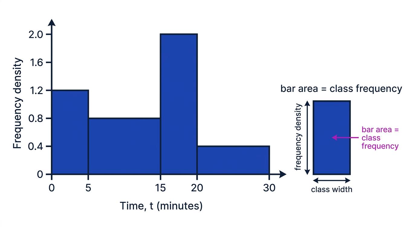
Area, not height
A taller histogram bar does not necessarily represent a larger frequency. You must compare the areas of the bars, especially when the class widths are unequal.
Recovering frequencies from a histogram
The histogram above has frequency densities 1.2, 0.8, 2.0 and 0.4 for class widths 5, 10, 5 and 10 respectively.
- For 0<t≤50<t\le50<t≤5, calculate the bar area: f=5×1.2=6f=5\times1.2=6f=5×1.2=6.
- For 5<t≤155<t\le155<t≤15, the frequency is f=10×0.8=8f=10\times0.8=8f=10×0.8=8.
- For 15<t≤2015<t\le2015<t≤20, the frequency is f=5×2.0=10f=5\times2.0=10f=5×2.0=10.
- For 20<t≤3020<t\le3020<t≤30, the frequency is f=10×0.4=4f=10\times0.4=4f=10×0.4=4.
- Therefore, the total frequency is 6+8+10+4=286+8+10+4=286+8+10+4=28.
Reading height as frequency
Do not copy the frequency density from the vertical axis and call it the frequency. Multiply it by the class width to find the bar’s area.
Estimating the mean from a histogram
The mean measures the central location of a distribution. For grouped data, you assume that every observation in a class is located at the class midpoint.
If midpoint xix_ixi represents a class with frequency fif_ifi, then the estimated mean is
xˉ=∑fixi∑fi.\bar{x}=\frac{\sum f_i x_i}{\sum f_i}.xˉ=∑fi∑fixi.Here, ∑fi\sum f_i∑fi is the total frequency and ∑fixi\sum f_i x_i∑fixi is the sum of each midpoint multiplied by its frequency.
Estimating the mean from histogram data
Use the frequencies recovered from the histogram: 6, 8, 10 and 4. The corresponding midpoints are 2.5, 10, 17.5 and 25.
-
Multiply each midpoint by its frequency:
∑fixi=6(2.5)+8(10)+10(17.5)+4(25)=370.\sum f_i x_i =6(2.5)+8(10)+10(17.5)+4(25) =370.∑fixi=6(2.5)+8(10)+10(17.5)+4(25)=370. -
Use the total frequency, ∑fi=28\sum f_i=28∑fi=28, in the grouped-mean formula:
xˉ=37028=13.214…\bar{x}=\frac{370}{28}=13.214\ldotsxˉ=28370=13.214… -
Therefore, the estimated mean time is approximately 13.2 minutes.
A quick reasonableness check
The estimated mean should lie within the overall range of the data. It will usually be pulled towards the side of the histogram containing more area or a longer tail.
Estimating the standard deviation
The standard deviation measures how spread out the data are around the mean.
- A small standard deviation means values are concentrated close to the mean.
- A large standard deviation means values are more widely dispersed.
For grouped data, using class midpoints gives
sx=∑fixi2∑fi−xˉ2.s_x=\sqrt{\frac{\sum f_i x_i^2}{\sum f_i}-\bar{x}^2}.sx=∑fi∑fixi2−xˉ2.As with the estimated mean, this is only an estimate because the exact values within each class are unknown.
Estimating the standard deviation
Continue with the same histogram, where ∑fi=28\sum f_i=28∑fi=28, ∑fixi=370\sum f_i x_i=370∑fixi=370 and xˉ=37028\bar{x}=\frac{370}{28}xˉ=28370.
-
Calculate the sum of frequency multiplied by squared midpoint:
∑fixi2=6(2.52)+8(102)+10(17.52)+4(252)=6400.\begin{aligned} \sum f_i x_i^2 &=6(2.5^2)+8(10^2)+10(17.5^2)+4(25^2)\\ &=6400. \end{aligned}∑fixi2=6(2.52)+8(102)+10(17.52)+4(252)=6400. -
Substitute into the variance expression:
∑fixi2∑fi−xˉ2=640028−(37028)2≈53.94.\frac{\sum f_i x_i^2}{\sum f_i}-\bar{x}^2 =\frac{6400}{28}-\left(\frac{370}{28}\right)^2 \approx53.94.∑fi∑fixi2−xˉ2=286400−(28370)2≈53.94. -
Take the positive square root:
sx≈53.94≈7.34.s_x\approx\sqrt{53.94}\approx7.34.sx≈53.94≈7.34. -
Therefore, the estimated standard deviation is approximately 7.34 minutes.
Forgetting to square the midpoint
The second total is ∑fixi2\sum f_i x_i^2∑fixi2, not (∑fixi)2\left(\sum f_i x_i\right)^2(∑fixi)2. Square each midpoint before multiplying it by its class frequency.
Rounding too early
Keep the mean and intermediate totals unrounded until the final step. Early rounding can noticeably change the calculated standard deviation.
Reading the mean and spread from a histogram
The mean can be thought of as the balance point of the histogram when each bar’s area is treated as its weight.
For a roughly symmetrical, single-peaked histogram, the mean is usually near the centre of symmetry. For a skewed histogram, the mean is pulled towards the long tail.
The standard deviation describes horizontal spread:
- Bars concentrated close to the mean suggest a smaller standard deviation.
- Substantial area far from the mean suggests a larger standard deviation.
- Two histograms can have the same mean but different standard deviations.
- Two histograms can have similar standard deviations but different means.
Position and spread
Changing the mean shifts the centre of a distribution. Changing the standard deviation alters how dispersed the data are around that centre.
You cannot normally obtain the exact mean or standard deviation merely by looking at a histogram. You need numerical scales and enough information to determine the class frequencies.
How transformations affect the histogram
If a constant aaa is added to every value, the histogram shifts horizontally by aaa. The mean increases by aaa, but the standard deviation is unchanged:
yˉ=xˉ+a,sy=sx.\bar{y}=\bar{x}+a,\qquad s_y=s_x.yˉ=xˉ+a,sy=sx.If every value is multiplied by a positive constant bbb, all horizontal distances are scaled by bbb. Both the mean and standard deviation are multiplied by bbb:
yˉ=bxˉ,sy=bsx.\bar{y}=b\bar{x},\qquad s_y=bs_x.yˉ=bxˉ,sy=bsx.Transforming the mean and standard deviation
A distribution has mean 13.2 and standard deviation 7.34. A new variable is defined by y=2x+5y=2x+5y=2x+5.
-
Apply the multiplication and addition to the mean:
yˉ=2(13.2)+5=31.4.\bar{y}=2(13.2)+5=31.4.yˉ=2(13.2)+5=31.4. -
Multiplying by 2 doubles the standard deviation, while adding 5 does not affect it:
sy=2(7.34)=14.68.s_y=2(7.34)=14.68.sy=2(7.34)=14.68. -
The transformed distribution therefore has mean 31.4 and standard deviation 14.68.
In the exam
- Check whether the vertical axis shows frequency or frequency density; for a histogram with unequal class widths, use bar area to recover frequency.
- Record the class widths, frequencies and midpoints carefully, then calculate ∑fi\sum f_i∑fi, ∑fixi\sum f_i x_i∑fixi and ∑fixi2\sum f_i x_i^2∑fixi2.
- State that answers found from grouped data are estimates, keep full calculator values during the working, and round only the final result.
Check yourself
- Why is the height of a histogram bar not generally equal to its frequency?
- How would you estimate the mean from class boundaries and frequency densities?
- What happens to the mean and standard deviation when every observation is increased by 10?
