

What you'll learn
- How a sample can provide evidence about a wider population.
- Why sampling variation means that conclusions are never completely certain.
- How a hypothesis test uses a critical region to make a decision.
- Why the significance level measures the probability of incorrectly rejecting the null hypothesis.
From populations to samples
A population is the complete set of individuals or observations that you want to investigate. A sample is a smaller group selected from that population.
For example, if a manufacturer wants to investigate the lifetime of every battery it produces, all its batteries form the population. A group of 100 tested batteries would be a sample.
Usually, measuring the entire population would be too expensive, slow or destructive. Instead, you collect sample data and use it to draw a conclusion about the population.
Statistical inference
Statistical inference is the process of using information from a sample to draw conclusions about the population from which it was taken.
The conclusion is only as reliable as the sample. Ideally, the sample should be randomly selected and representative of the population. A biased sample may lead to a misleading inference, even if every calculation is correct.
Making an inference from a sample
A factory claims that 10% of its components are defective. In a random sample of 40 components, 9 are defective.
-
The population is all components produced by the factory, while the 40 inspected components form the sample.
-
The sample proportion that is defective is
940=0.225.\frac{9}{40}=0.225.409=0.225. -
Since 22.5% is noticeably greater than the claimed 10%, the sample provides some evidence that the true population proportion may be greater than 10%.
-
However, this difference could have arisen through chance sampling variation. A hypothesis test is needed to judge whether the result is sufficiently unusual.
Sampling variation
Different random samples from the same population will usually produce different results. This natural difference between samples is called sampling variation.
Suppose a fair coin is tossed 20 times. You would not expect every set of 20 tosses to contain exactly 10 heads. Results such as 8, 11 or 12 heads are entirely plausible even though the probability of heads remains p=0.5p=0.5p=0.5.
This creates the central question in hypothesis testing:
Is the observed sample result just ordinary sampling variation, or is it strong evidence that the population assumption is wrong?
Evidence, not certainty
A sample does not prove a statement about a population. It provides evidence that may or may not be strong enough to reject an assumed model.
The null and alternative hypotheses
A statistical hypothesis is a statement about a population parameter, such as a population proportion or mean.
The null hypothesis, written H0H_0H0, is the initial assumption being tested. It usually represents no change, no effect or the stated population model.
The alternative hypothesis, written H1H_1H1, describes the possibility for which you are seeking evidence.
For example, if a coin is claimed to have probability p=0.5p=0.5p=0.5 of landing heads, but you suspect that it favours heads, the hypotheses are
H0:p=0.5andH1:p>0.5.H_0:p=0.5 \qquad\text{and}\qquad H_1:p>0.5.H0:p=0.5andH1:p>0.5.A test is one-tailed if H1H_1H1 looks in one specified direction, such as p>0.5p>0.5p>0.5 or p<0.5p<0.5p<0.5. It is two-tailed if H1H_1H1 allows differences in either direction, such as p≠0.5p\neq0.5p=0.5.
Choosing the alternative after seeing the data
The alternative hypothesis must come from the wording and context of the investigation, not from the direction in which the sample happens to differ.
Test statistics and unusual results
A test statistic is a quantity calculated from the sample and used to carry out the test. For a binomial test, it is often the number of successes, written XXX.
You first assume that H0H_0H0 is true. This gives a probability distribution for the test statistic. You then ask how likely it would be, under this assumption, to obtain a result at least as extreme as the observed one.
If that probability is sufficiently small, the sample result is considered significant: it would be difficult to explain by chance variation alone if H0H_0H0 were true.
Critical region
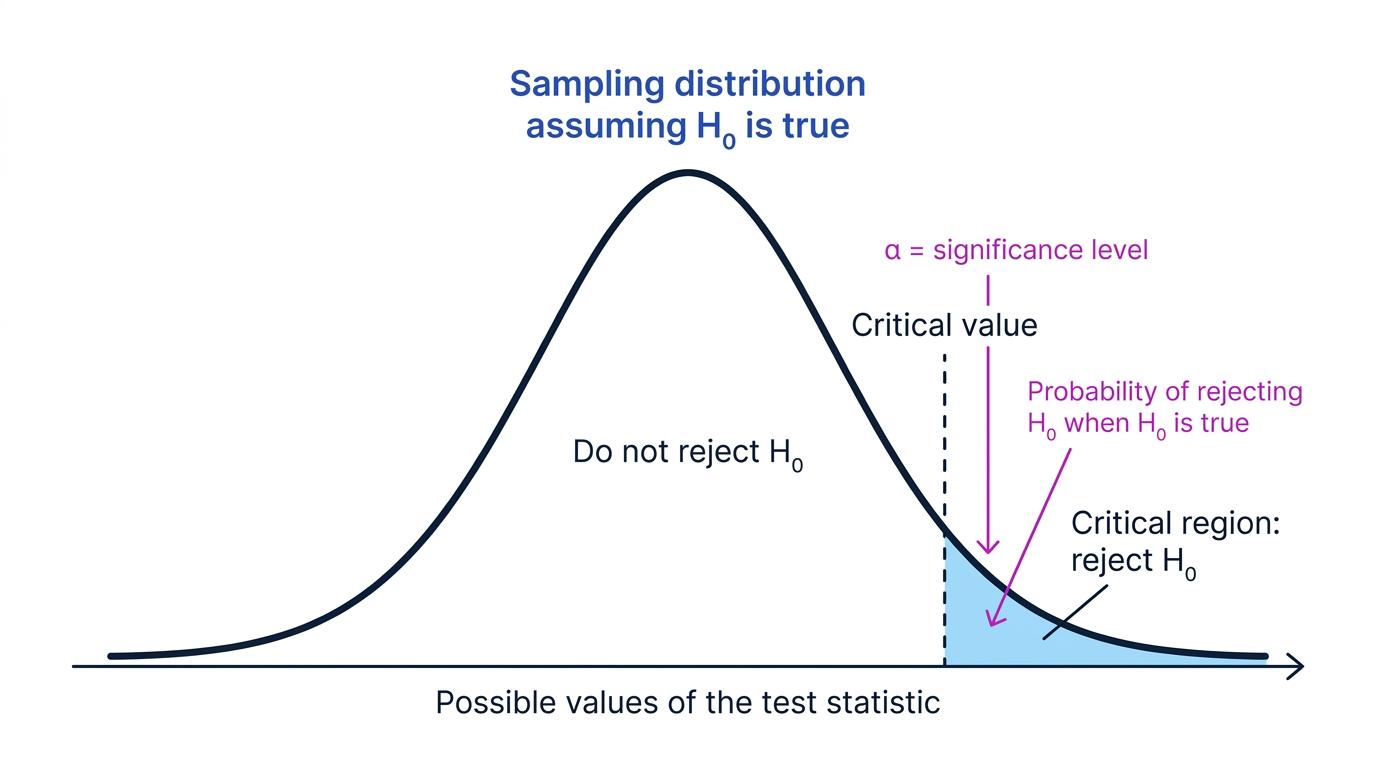
The critical region is the set of values of the test statistic that lead to the rejection of H0H_0H0. Its boundary is called a critical value.
The significance level is represented by the shaded tail area under the sampling distribution when H0H_0H0 is true.
Significance level
The significance level is the probability of rejecting H0H_0H0 when H0H_0H0 is actually true. It is commonly denoted by α\alphaα.
For example, a 5% significance level means that the testing procedure has at most about a 5% probability of rejecting a true null hypothesis.
Type I error
A Type I error occurs when you reject the null hypothesis even though it is true. Therefore,
P(Type I error)=α.P(\text{Type I error})=\alpha.P(Type I error)=α.This probability is calculated assuming that H0H_0H0 is true. It is not the probability that H0H_0H0 itself is true, and it is not the probability that your final conclusion is wrong.
Misinterpreting 5% significance
A 5% significance level does not mean there is a 5% probability that H0H_0H0 is true. In this method, H0H_0H0 is treated as fixed; the probability describes how the sample behaves when H0H_0H0 is true.
Constructing a critical region
Suppose a fair coin is tossed 10 times and XXX is the number of heads. Under the null hypothesis,
X∼B(10,0.5).X\sim\operatorname{B}(10,0.5).X∼B(10,0.5).If the alternative is that the coin favours heads, large values of XXX count against H0H_0H0. The critical region must therefore be in the upper tail.
Finding an upper-tail critical region
Find a critical region for a test at the 5% significance level.
-
Since H1:p>0.5H_1:p>0.5H1:p>0.5, consider values of the form X≥cX\ge cX≥c, where ccc is the critical value.
-
Calculate the probability of the most extreme upper-tail result:
P(X≥10)=P(X=10)=(0.5)10≈0.000977.P(X\ge10)=P(X=10)=(0.5)^{10}\approx0.000977.P(X≥10)=P(X=10)=(0.5)10≈0.000977. -
Widen the region by including 9 heads:
P(X≥9)=P(X=9)+P(X=10)=(109)(0.5)10+(0.5)10=111024≈0.0107.\begin{aligned} P(X\ge9) &=P(X=9)+P(X=10)\\ &=\binom{10}{9}(0.5)^{10}+(0.5)^{10}\\ &=\frac{11}{1024}\\ &\approx0.0107. \end{aligned}P(X≥9)=P(X=9)+P(X=10)=(910)(0.5)10+(0.5)10=102411≈0.0107. -
Including 8 heads would give
P(X≥8)=561024≈0.0547,P(X\ge8)=\frac{56}{1024}\approx0.0547,P(X≥8)=102456≈0.0547,which exceeds 0.05. Therefore the largest permissible critical region is X≥9X\ge9X≥9.
-
The actual significance level is approximately 1.07%, because this is the probability of entering the critical region when H0H_0H0 is true.
For a discrete distribution such as the binomial distribution, the tail probabilities increase in jumps. It may therefore be impossible to create a critical region whose probability is exactly 5%.
Nominal and actual significance
A test described as being at the 5% significance level should have a critical-region probability no greater than 5%. For a discrete distribution, the actual significance level may be smaller.
Making the decision
Once the critical region has been established, compare the observed test statistic with it:
- If the result lies inside the critical region, reject H0H_0H0. There is sufficient evidence to support H1H_1H1 at the stated significance level.
- If the result lies outside the critical region, do not reject H0H_0H0. There is insufficient evidence to support H1H_1H1 at the stated significance level.
Drawing a contextual conclusion
Using the test above, suppose the coin produces 9 heads in 10 tosses.
- The observed value is x=9x=9x=9.
- Since 9≥99\ge99≥9, the result lies in the critical region.
- Reject H0H_0H0. There is sufficient evidence at the 5% significance level to suggest that the coin favours heads.
You should say “do not reject H0H_0H0”, rather than “accept H0H_0H0”. A non-significant result does not prove that the null hypothesis is true; the sample may simply contain too little evidence to reject it.
Think like a cautious statistician
A significant result means “unlikely under H0H_0H0”, not “impossible under H0H_0H0”. Even a correctly performed test can reject a true null hypothesis.
Changing the significance level
A smaller significance level, such as 1% rather than 5%, demands stronger evidence before H0H_0H0 is rejected. The critical region becomes smaller, so a Type I error is less likely.
A larger significance level makes rejection easier, but increases the probability of rejecting a true H0H_0H0.
The choice of level depends on context. When a false rejection could have serious consequences, a lower significance level may be appropriate.
In the exam
- Identify the population parameter and write H0H_0H0 and H1H_1H1 using the correct equality and direction.
- Work under the assumption that H0H_0H0 is true, and place the critical region in the tail or tails indicated by H1H_1H1.
- Check that the probability of the critical region does not exceed the stated significance level.
- Compare the observed statistic with the critical region, then state “reject” or “do not reject” H0H_0H0.
- Finish in context using “sufficient evidence” or “insufficient evidence”; do not claim that either hypothesis has been proved.
Check yourself
- What is the difference between a population and a sample?
- What does a 1% significance level mean in terms of rejecting H0H_0H0?
- Why might the actual significance level of a binomial test be less than its stated significance level?
