

What you'll learn
- How to distinguish between discrete and continuous random variables.
- How to decide whether a binomial or Normal distribution is a suitable model.
- How to justify your choice using the context rather than relying only on keywords.
- How to recognise assumptions that make either model inappropriate.
Probability distributions as models
A random variable is a variable whose value depends on the outcome of a random process. It is usually represented by a capital letter such as XXX.
A probability distribution describes the possible values of a random variable and how likely those values are.
In real situations, a probability distribution is a mathematical model. It simplifies reality by making assumptions. A model does not need to describe every detail perfectly, but its assumptions should be reasonable for the context.
Discrete and continuous random variables
A discrete random variable takes separate, countable values, such as 0, 1, 2, and so on. A continuous random variable can take any value within an interval.
For example:
- The number of defective components in a box is discrete.
- The mass of a component is continuous.
- The number of customers arriving late is discrete.
- The time taken by a customer is continuous.
Classifying recorded measurements
A continuous quantity can be rounded when it is recorded. A person's height measured to the nearest centimetre is still fundamentally continuous because the true height could take any value within a range.
Classifying random variables
Decide whether each variable is discrete or continuous: the number of goals in a match, and the lifetime of a battery.
- The number of goals is obtained by counting and can take values such as 0, 1, 2, and so on. It is therefore discrete.
- A battery lifetime is obtained by measuring time and could, in principle, take any positive value. It is therefore continuous.
- This suggests that a discrete model might be considered for the goal count, whereas a continuous model might be considered for the battery lifetime. It does not yet prove that a particular distribution is suitable.
The binomial distribution
The binomial distribution models the number of successes in a fixed number of repeated trials.
If XXX has a binomial distribution, write
X∼B(n,p),X \sim \mathrm{B}(n,p),X∼B(n,p),where nnn is the number of trials and ppp is the probability of success on each trial.
Conditions for a binomial model
A binomial model requires:
- a fixed number nnn of trials;
- exactly two possible outcomes on each trial, labelled success and failure;
- independent trials, meaning one result does not affect another;
- a constant probability of success ppp on every trial.
The word success does not necessarily mean something desirable. A defective component, a missed train or an incorrect answer can all be defined as a success if that is the outcome being counted.
Selecting a binomial model
A fair coin is tossed 20 times. Let XXX be the number of heads. Decide whether a binomial model is appropriate.
- There is a fixed number of trials, with n=20n=20n=20.
- Each trial has two relevant outcomes: head or not head. If a head is called a success, its probability is constant at p=12p=\frac12p=21.
- The result of one toss does not affect another, so independence is reasonable.
- All four binomial conditions are satisfied, so an appropriate model is
When the binomial model is inappropriate
A binomial model should not be used just because a question involves counting. You must check its assumptions.
It may be inappropriate when:
- the number of trials is not fixed;
- there are more than two relevant outcomes per trial;
- the probability of success changes;
- trials are dependent;
- the variable is not counting successes.
Rejecting a binomial model
Five cards are drawn from a standard pack without replacement. Let XXX be the number of aces drawn. Decide whether XXX should be modelled by a binomial distribution.
- There is a fixed number of trials, and each draw can be classified as ace or not ace.
- However, the cards are drawn without replacement. The probability of an ace changes after every draw. For example, it begins at 452\frac{4}{52}524, but after an ace is drawn it becomes 351\frac{3}{51}513.
- The draws are also dependent because the result of one draw changes the composition of the pack.
- Therefore, an exact binomial model is not appropriate.
Sampling without replacement
Sampling without replacement creates dependence. If the sample is very small compared with a large population, a binomial model may sometimes be a reasonable approximation, but you should state why the dependence is negligible.
The Normal distribution
The Normal distribution is a continuous probability distribution with a symmetric, bell-shaped density curve.
If XXX has a Normal distribution, write
X∼N(μ,σ2),X \sim \mathrm{N}(\mu,\sigma^2),X∼N(μ,σ2),where μ\muμ is the mean and σ2\sigma^2σ2 is the variance. The standard deviation is σ\sigmaσ.
A Normal model is often reasonable for continuous measurements that:
- cluster around one central value;
- are approximately symmetric;
- have a single peak;
- become less common further from the centre;
- are not strongly affected by outliers or strict boundaries.
Shape of a Normal model
A Normal distribution is continuous, symmetric about its mean, and defined over all real values. Its mean, median and mode are equal.
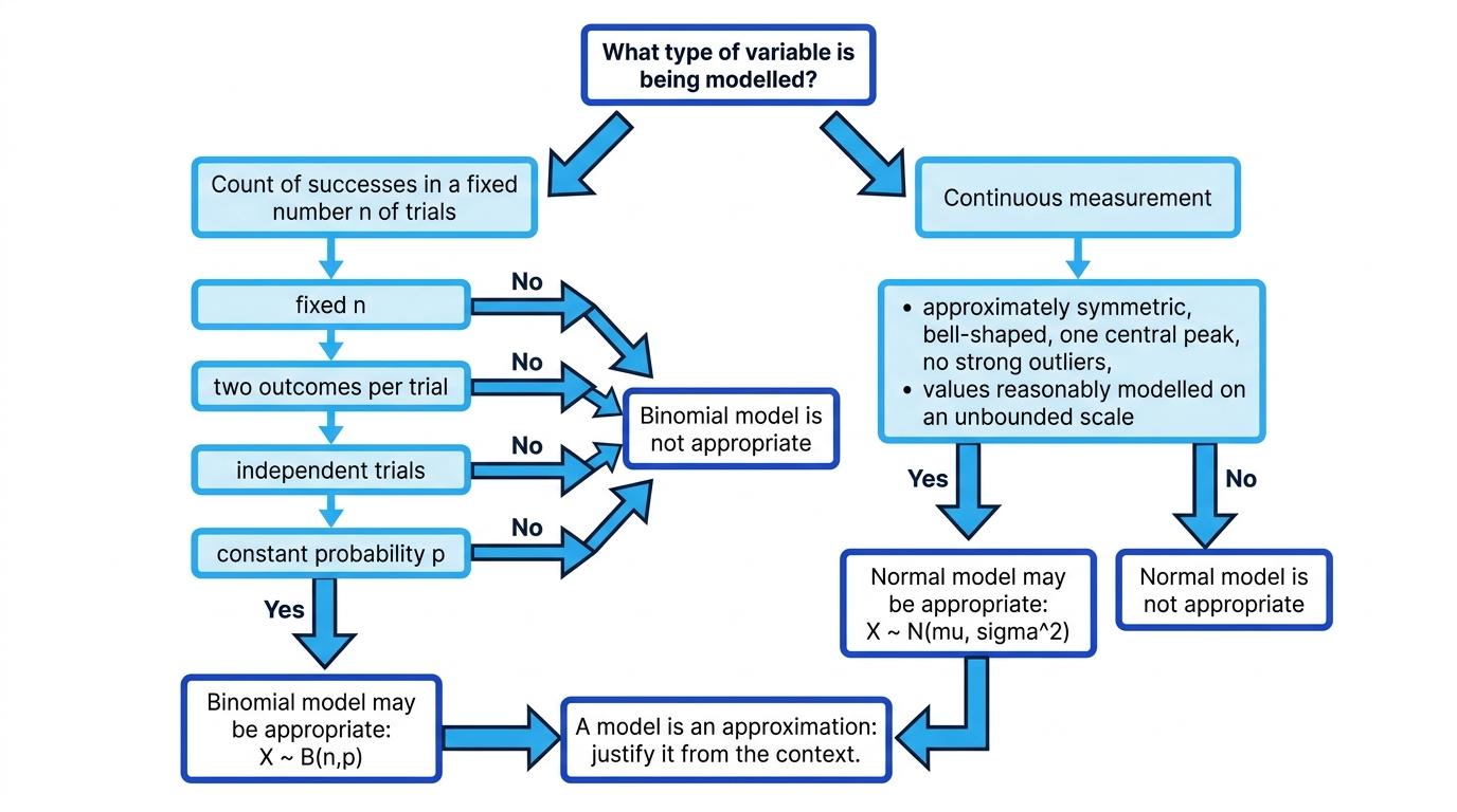
The following decision process helps you connect the type of variable and the assumptions to a possible model.
Selecting a Normal model
The masses of loaves produced by a machine vary around a target of 800 g. The distribution is approximately symmetric, has one central peak and has no obvious outliers. Decide whether a Normal model is reasonable.
- Mass is a continuous variable, so a continuous distribution is required.
- Small variations in ingredients and production conditions can act in both directions around the target, making an approximately symmetric shape plausible.
- The stated single peak and lack of strong outliers are consistent with a bell-shaped distribution.
- A Normal model is therefore reasonable, provided the spread is small enough that impossible negative masses have negligible probability.
When the Normal model is inappropriate
The Normal distribution extends from negative infinity to positive infinity. It can therefore assign probability to impossible values, such as negative masses or times.
This is not automatically a problem. If the mean is many standard deviations above zero, the probability assigned to negative values may be negligible. However, it matters when a boundary is close to the centre of the distribution.
A Normal model may also be unsuitable when the data are:
- strongly skewed, with a much longer tail on one side;
- bimodal, meaning they have two distinct peaks;
- affected by substantial outliers;
- discrete with only a few possible values;
- bounded in a way that conflicts seriously with the Normal curve.
Rejecting a Normal model
A website records the amount spent by each customer during a visit. Most customers spend a small amount, but a few spend several hundred pounds. Decide whether a Normal model is appropriate.
- Amount spent is treated as continuous, so being continuous alone does not rule out a Normal model.
- The few very large purchases create a long right-hand tail, so the distribution is strongly positively skewed rather than symmetric.
- Spending cannot be negative, and this lower boundary may be important because many observations are close to zero.
- A Normal model is therefore unlikely to be appropriate.
Assuming every continuous variable is Normal
Continuous does not mean Normal. You must also consider symmetry, shape, outliers and whether the possible values are compatible with an unbounded Normal model.
Choosing between the models
Start by identifying exactly what XXX represents.
- If XXX counts successes in repeated trials, test all four binomial conditions.
- If XXX is a continuous measurement, consider whether a symmetric, bell-shaped Normal model is plausible.
- If neither set of assumptions is reasonable, say that neither model is appropriate.
Your justification should refer directly to the context. For example, write “the probability of a defective item may change as the machine warms up”, rather than merely writing “ppp is not constant”.
Comparing possible models
A researcher measures the waiting time, in minutes, until the next bus arrives. Should this be modelled by a binomial or Normal distribution?
- Waiting time is continuous and does not count successes in a fixed number of trials, so a binomial model is inappropriate.
- Waiting time cannot be negative and may have a long right-hand tail when buses are delayed, so symmetry should not be assumed.
- Unless there is evidence that waiting times are approximately symmetric with a suitable mean and spread, a Normal model is also questionable.
- The correct conclusion may therefore be that neither model is justified by the information given.
In the exam
- Define the random variable clearly and decide whether it is discrete or continuous.
- For a binomial model, check fixed nnn, two outcomes, independence and constant ppp.
- For a Normal model, check continuity, approximate symmetry, one central peak, outliers and important boundaries.
- Justify each assumption using details from the context, not just the name of the condition.
- Be willing to conclude that neither distribution is appropriate.
Check yourself
- Why is sampling without replacement often inconsistent with a binomial model?
- What features of a data distribution would make a Normal model doubtful?
- A variable is continuous. What further information would you need before selecting a Normal distribution?
