

What you'll learn
- How logarithms turn certain non-linear relationships into straight-line equations.
- Which quantities to plot for models of the form y=axny=ax^ny=axn and y=kbxy=kb^xy=kbx.
- How to estimate the parameters aaa, nnn, kkk and bbb from a line of best fit.
- How to decide which model is more suitable for a set of data.
Prerequisites
Straight-line equations
A straight line can be written as
Y=mX+c,Y=mX+c,Y=mX+c,where:
- XXX is the quantity on the horizontal axis.
- YYY is the quantity on the vertical axis.
- mmm is the gradient, which measures the steepness of the line.
- ccc is the vertical intercept, where the line crosses the vertical axis.
For two points (X1,Y1)(X_1,Y_1)(X1,Y1) and (X2,Y2)(X_2,Y_2)(X2,Y2) on the line,
m=Y2−Y1X2−X1.m=\frac{Y_2-Y_1}{X_2-X_1}.m=X2−X1Y2−Y1.This familiar structure is the key to estimating parameters: you transform the variables until the model looks like Y=mX+cY=mX+cY=mX+c.
Logarithm laws
You need three logarithm laws:
log(uv)=logu+logv,log(ur)=rlogu,log(bx)=xlogb.\begin{aligned} \log(uv)&=\log u+\log v,\\ \log(u^r)&=r\log u,\\ \log(b^x)&=x\log b. \end{aligned}log(uv)log(ur)log(bx)=logu+logv,=rlogu,=xlogb.In this topic, log\loglog usually means the base-10 logarithm. You could use natural logarithms, written ln\lnln, instead, but you must use the same base throughout.
Linearisation
Linearisation is the process of transforming a non-linear relationship into a straight-line equation. It allows you to estimate unknown parameters using a graph.
Why logarithms help
Logarithms bring powers down in front and turn multiplication into addition. This reveals the gradient and intercept of a hidden straight line.
Power relationships
A power relationship has the form
y=axn,y=ax^n,y=axn,where aaa and nnn are constant parameters. The parameter nnn is the power, or index, applied to xxx.
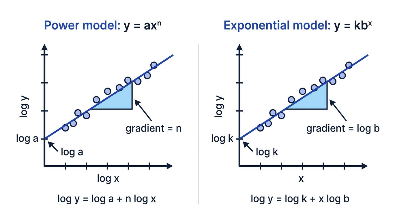
The graph of yyy against xxx is usually curved, so its gradient is not constant. Take logarithms of both sides:
logy=log(axn)=loga+log(xn)=loga+nlogx.\begin{aligned} \log y&=\log(ax^n)\\ &=\log a+\log(x^n)\\ &=\log a+n\log x. \end{aligned}logy=log(axn)=loga+log(xn)=loga+nlogx.Reordering gives
logy=nlogx+loga.\log y=n\log x+\log a.logy=nlogx+loga.Compare this with Y=mX+cY=mX+cY=mX+c:
- Plot logy\log ylogy vertically against logx\log xlogx horizontally.
- The gradient is nnn.
- The vertical intercept is loga\log aloga.
- Therefore, a=10intercepta=10^{\text{intercept}}a=10intercept when base-10 logarithms are used.
Estimating a power model
A plot of logy\log ylogy against logx\log xlogx produces a line of best fit passing through the points (0.20,0.72)(0.20,0.72)(0.20,0.72) and (0.80,1.98)(0.80,1.98)(0.80,1.98). Its vertical intercept is approximately 0.300.300.30. Estimate aaa and nnn.
-
Calculate the gradient of the line:
n=1.98−0.720.80−0.20=1.260.60=2.1.n=\frac{1.98-0.72}{0.80-0.20} =\frac{1.26}{0.60} =2.1.n=0.80−0.201.98−0.72=0.601.26=2.1.The gradient represents nnn, so n≈2.1n\approx2.1n≈2.1.
-
Use the intercept loga≈0.30\log a\approx0.30loga≈0.30:
a≈100.30≈2.00.a\approx10^{0.30}\approx2.00.a≈100.30≈2.00. -
Substitute both estimates into the original model:
y≈2.00x2.1.y\approx2.00x^{2.1}.y≈2.00x2.1.
Forgetting the inverse logarithm
The intercept is loga\log aloga, not aaa. If the intercept is ccc, you must calculate a=10ca=10^ca=10c for base-10 logarithms, or a=eca=e^ca=ec if natural logarithms were used.
Exponential relationships
An exponential relationship has the form
y=kbx,y=kb^x,y=kbx,where kkk and bbb are constant parameters and the variable xxx appears in the exponent.
Take logarithms:
logy=log(kbx)=logk+log(bx)=logk+xlogb.\begin{aligned} \log y&=\log(kb^x)\\ &=\log k+\log(b^x)\\ &=\log k+x\log b. \end{aligned}logy=log(kbx)=logk+log(bx)=logk+xlogb.Therefore,
logy=(logb)x+logk.\log y=(\log b)x+\log k.logy=(logb)x+logk.Compare this with Y=mX+cY=mX+cY=mX+c:
- Plot logy\log ylogy vertically against xxx horizontally.
- The gradient is logb\log blogb.
- The vertical intercept is logk\log klogk.
- Therefore, b=10gradientb=10^{\text{gradient}}b=10gradient and k=10interceptk=10^{\text{intercept}}k=10intercept for base-10 logarithms.
Notice the crucial difference: for a power model you log both variables, but for an exponential model you log only yyy.
Estimating an exponential model
A plot of logy\log ylogy against xxx gives a line of best fit with gradient 0.1760.1760.176 and vertical intercept 0.6990.6990.699. Estimate kkk and bbb.
-
Since the intercept is logk\log klogk,
k=100.699≈5.00.k=10^{0.699}\approx5.00.k=100.699≈5.00. -
Since the gradient is logb\log blogb,
b=100.176≈1.50.b=10^{0.176}\approx1.50.b=100.176≈1.50. -
Substitute the estimates into the original model:
y≈5.00(1.50)x.y\approx5.00(1.50)^x.y≈5.00(1.50)x.
Using the gradient directly
For y=kbxy=kb^xy=kbx, the gradient is logb\log blogb, not bbb. A gradient of 0.1760.1760.176 gives b=100.176b=10^{0.176}b=100.176, not b=0.176b=0.176b=0.176.
Working from a data set
A question may give measured values of xxx and $y` rather than a ready-made logarithmic graph. You should:
- Decide which model is being tested.
- Calculate the required transformed values.
- Plot the transformed coordinates.
- Draw a straight line of best fit.
- use two well-separated points on your line to find its gradient.
- Read or calculate the intercept, then convert it back using an inverse logarithm.
For y=axny=ax^ny=axn, calculate logx\log xlogx and $\log y`.
For y=kbxy=kb^xy=kbx, keep xxx unchanged and calculate only $\log y`.
Transforming power-model data
Suppose two observations are (x,y)=(2,12.4)(x,y)=(2,12.4)(x,y)=(2,12.4) and (5,78.1)(5,78.1)(5,78.1), and a power model is proposed.
-
Transform both coordinates using base-10 logarithms:
(log2,log12.4)≈(0.301,1.093),(log5,log78.1)≈(0.699,1.893).\begin{aligned} (\log 2,\log 12.4)&\approx(0.301,1.093),\\ (\log 5,\log 78.1)&\approx(0.699,1.893). \end{aligned}(log2,log12.4)(log5,log78.1)≈(0.301,1.093),≈(0.699,1.893). -
Use the transformed points to estimate the gradient:
n≈1.893−1.0930.699−0.301=0.8000.398≈2.01.n\approx\frac{1.893-1.093}{0.699-0.301} =\frac{0.800}{0.398} \approx2.01.n≈0.699−0.3011.893−1.093=0.3980.800≈2.01. -
Substitute one transformed point into logy=nlogx+loga\log y=n\log x+\log alogy=nlogx+loga:
1.093≈2.01(0.301)+loga,loga≈0.488.\begin{aligned} 1.093&\approx2.01(0.301)+\log a,\\ \log a&\approx0.488. \end{aligned}1.093loga≈2.01(0.301)+loga,≈0.488.Hence,
a≈100.488≈3.08,a\approx10^{0.488}\approx3.08,a≈100.488≈3.08,giving the estimated model y≈3.08x2.01y\approx3.08x^{2.01}y≈3.08x2.01.
Use the best-fit line
When data are scattered, calculate the gradient using two well-separated points on your line of best fit. They do not need to be original data points.
Choosing between the models
The appropriate transformation depends on the proposed relationship:
- If plotting logy\log ylogy against logx\log xlogx gives an approximately straight line, a power model y=axny=ax^ny=axn is supported.
- If plotting logy\log ylogy against xxx gives an approximately straight line, an exponential model y=kbxy=kb^xy=kbx is supported.
A perfect line is unlikely with real data. You are looking for points that lie reasonably close to a straight line without a systematic curved pattern.
Straightness tests the model
The model whose required logarithmic plot is closest to a straight line is generally the more suitable model for the data.
Restrictions and interpretation
Logarithms of zero or negative numbers are not defined in real-number A-level mathematics. The basic method therefore requires the quantities being logged to be positive.
For the usual models in this topic:
a>0,k>0,b>0,a>0,\qquad k>0,\qquad b>0,a>0,k>0,b>0,with x>0x>0x>0 and y>0y>0y>0 when plotting logx\log xlogx against $\log y`.
If 0<b<10<b<10<b<1, then $\log b<0`, so the exponential graph has a negative gradient. This represents exponential decay.
If n<0n<0n<0, the log-log graph for a power model also has a negative gradient.
Non-positive data
You cannot directly calculate logx\log xlogx or logy\log ylogy when the relevant value is zero or negative. Do not ignore such values without explaining why the proposed transformation cannot use them.
In the exam
- Write the logarithmic equation before identifying the gradient and intercept.
- Label transformed axes precisely: use logy\log ylogy against logx\log xlogx for y=axny=ax^ny=axn, but logy\log ylogy against xxx for y=kbxy=kb^xy=kbx.
- Use a large gradient triangle on the line of best fit and keep extra calculator figures until the final answer.
- Convert logarithmic values back correctly, then state the estimated model in its original form.
Check yourself
- For y=axny=ax^ny=axn, what should you plot, and what do the gradient and intercept represent?
- A plot of logy\log ylogy against xxx has gradient −0.301-0.301−0.301 and intercept 1.201.201.20. How would you estimate bbb and kkk?
- How could transformed graphs help you choose between a power model and an exponential model?
