

What you'll learn
- How to translate a differential equation and its solution into the language of a real problem.
- How to interpret gradients, constants, limiting values and long-term behaviour.
- How differential equations connect displacement, velocity and acceleration in kinematics.
- How to identify assumptions and limitations in a mathematical model.
Prerequisites: rates of change
A derivative measures the instantaneous rate at which one quantity changes with respect to another.
If a quantity yyy depends on time ttt, then dydt\frac{dy}{dt}dtdy is its rate of change at time ttt. On a graph of yyy against ttt, this derivative is the gradient of the curve.
- If dydt>0\frac{dy}{dt}>0dtdy>0, then yyy is increasing.
- If dydt<0\frac{dy}{dt}<0dtdy<0, then yyy is decreasing.
- If dydt=0\frac{dy}{dt}=0dtdy=0, then the graph has a stationary point or the quantity is at an equilibrium value.
Differential equation
A differential equation is an equation containing a derivative, such as dydt\frac{dy}{dt}dtdy, together with the quantity being modelled.
For example,
dydt=3y\frac{dy}{dt}=3ydtdy=3y
says that the rate of change of yyy is three times its current value. It describes a relationship between a quantity and the way that quantity changes.
Read the derivative in words
Before doing any algebra, translate dydt=f(y,t)\frac{dy}{dt}=f(y,t)dtdy=f(y,t) as “the rate of change of yyy is given by f(y,t)f(y,t)f(y,t)”.
Interpreting a population model
A population PPP, measured in thousands, is modelled by
dPdt=0.2P,\frac{dP}{dt}=0.2P,dtdP=0.2P,
where ttt is measured in years.
- Since PPP is a population and ttt is time, dPdt\frac{dP}{dt}dtdP represents the population’s instantaneous rate of change, in thousands per year.
- For any positive population, 0.2P>00.2P>00.2P>0. Therefore dPdt>0\frac{dP}{dt}>0dtdP>0, so the model predicts that the population increases.
- The rate is proportional to PPP. A larger population therefore produces a larger absolute increase per year; for example, when P=10P=10P=10, the rate is 222 thousand people per year.
What a solution represents
A solution of a differential equation is a function that satisfies the differential equation over a stated interval.
For example, a solution might be
y=Ce3t,y=Ce^{3t},y=Ce3t,
where CCC is an arbitrary constant. Differentiating gives
dydt=3Ce3t=3y,\frac{dy}{dt}=3Ce^{3t}=3y,dtdy=3Ce3t=3y,
so the function satisfies dydt=3y\frac{dy}{dt}=3ydtdy=3y.
A differential equation often has a whole family of solutions. An initial condition gives the value of the modelled quantity at a particular time and allows you to determine the arbitrary constant.
Initial condition
An initial condition is a known value such as y(0)=5y(0)=5y(0)=5, specifying the state of the system at a chosen starting time.
Using an initial population
The population model above has the general solution
P=Ae0.2t.P=Ae^{0.2t}.P=Ae0.2t.
Initially, the population is 10 thousand.
-
“Initially” means t=0t=0t=0, so the initial condition is P(0)=10P(0)=10P(0)=10.
-
Substitute this into the general solution:
10=Ae0.2(0)=A.10=Ae^{0.2(0)}=A.10=Ae0.2(0)=A.
Therefore A=10A=10A=10.
-
The particular solution is
P=10e0.2t.P=10e^{0.2t}.P=10e0.2t.
At time ttt, this gives the model’s predicted population in thousands.
Ignoring the meaning of the constant
An arbitrary constant is not just an algebraic extra. Once an initial condition is used, it records information about the system’s starting state.
Interpreting the shape of a solution
Once you have a solution, ask what it says about:
- the initial value;
- whether the quantity increases or decreases;
- how quickly it changes;
- any maximum, minimum or limiting value;
- its behaviour as time becomes large.
Suppose a velocity is modelled by
v=20(1−e−0.4t).v=20\left(1-e^{-0.4t}\right).v=20(1−e−0.4t).
At t=0t=0t=0, the velocity is zero. As ttt increases, e−0.4te^{-0.4t}e−0.4t decreases towards zero, so vvv increases towards 20 m s−120\text{ m s}^{-1}20 m s−1.
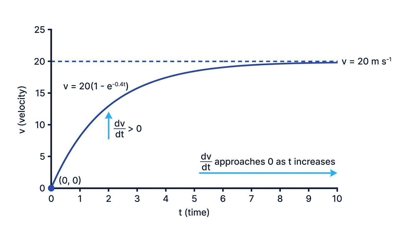
The line v=20v=20v=20 is a horizontal asymptote: the graph approaches this line as t→∞t\to\inftyt→∞.
Limiting value
A limiting value is the value approached by a modelled quantity as the independent variable tends towards a specified value, often as t→∞t\to\inftyt→∞.
Interpreting a limiting velocity
A particle’s velocity is
v=20(1−e−0.4t) m s−1,v=20\left(1-e^{-0.4t}\right)\text{ m s}^{-1},v=20(1−e−0.4t) m s−1,
where t≥0t\geq 0t≥0.
-
At the start,
v(0)=20(1−1)=0,v(0)=20(1-1)=0,v(0)=20(1−1)=0,
so the particle starts from rest.
-
Differentiate to find the acceleration:
a=dvdt=8e−0.4t.a=\frac{dv}{dt}=8e^{-0.4t}.a=dtdv=8e−0.4t.
Since this is positive for t≥0t\geq 0t≥0, the velocity is always increasing. However, the exponential factor decreases, so the acceleration becomes smaller.
-
As t→∞t\to\inftyt→∞, e−0.4t→0e^{-0.4t}\to 0e−0.4t→0, giving
v→20.v\to 20.v→20.
The model predicts that the particle approaches a limiting velocity of 20 m s−120\text{ m s}^{-1}20 m s−1.
-
The velocity never equals 20 at a finite time in this model. It becomes arbitrarily close to 20 as time increases.
Check the endpoints
Evaluate the solution at the initial time and examine its limit as t→∞t\to\inftyt→∞. These two checks often reveal most of the model’s physical meaning.
Equilibrium solutions
An equilibrium value is a value at which the modelled quantity has zero rate of change.
For an autonomous differential equation
dydt=f(y),\frac{dy}{dt}=f(y),dtdy=f(y),
equilibria are found by solving f(y)=0f(y)=0f(y)=0. If the quantity begins exactly at an equilibrium, the model predicts that it remains there.
Consider
dPdt=0.1P(1−P500).\frac{dP}{dt}=0.1P\left(1-\frac{P}{500}\right).dtdP=0.1P(1−500P).
The equilibria are P=0P=0P=0 and P=500P=500P=500.
Predicting behaviour near an equilibrium
Interpret the model for a positive population PPP.
- For 0<P<5000<P<5000<P<500, both PPP and 1−P5001-\frac{P}{500}1−500P are positive. Hence dPdt>0\frac{dP}{dt}>0dtdP>0, so the population increases.
- For P>500P>500P>500, the factor 1−P5001-\frac{P}{500}1−500P is negative. Hence dPdt<0\frac{dP}{dt}<0dtdP<0, so the population decreases.
- On either side of P=500P=500P=500, the population moves towards 500. Therefore 500 is a stable equilibrium and represents the model’s long-term limiting population.
- The value P=0P=0P=0 is also an equilibrium, but a small positive population moves away from zero. It is therefore an unstable equilibrium for positive populations.
Confusing zero rate with zero quantity
The condition dydt=0\frac{dy}{dt}=0dtdy=0 means the quantity is not changing at that instant. It does not usually mean that y=0y=0y=0.
Links to kinematics
In one-dimensional motion, let sss be displacement, vvv be velocity and aaa be acceleration. These are connected by
v=dsdt,a=dvdt=d2sdt2.v=\frac{ds}{dt}, \qquad a=\frac{dv}{dt}=\frac{d^2s}{dt^2}.v=dtds,a=dtdv=dt2d2s.
A differential equation involving vvv and dvdt\frac{dv}{dt}dtdv therefore describes how the acceleration depends on the particle’s velocity or on time.
Remember that velocity includes direction. A negative velocity means motion in the negative direction, while a negative acceleration does not necessarily mean that the particle is slowing down.
Interpreting velocity and acceleration
A particle has velocity
v=6−10e−2t m s−1,v=6-10e^{-2t}\text{ m s}^{-1},v=6−10e−2t m s−1,
for t≥0t\geq 0t≥0.
-
Initially,
v(0)=6−10=−4 m s−1,v(0)=6-10=-4\text{ m s}^{-1},v(0)=6−10=−4 m s−1,
so the particle initially moves in the negative direction.
-
Its acceleration is
a=dvdt=20e−2t m s−2,a=\frac{dv}{dt}=20e^{-2t}\text{ m s}^{-2},a=dtdv=20e−2t m s−2,
which is positive. While v<0v<0v<0, velocity and acceleration have opposite signs, so the particle slows down.
-
The particle changes direction when v=0v=0v=0:
6−10e−2t=0e−2t=35t=12ln(53).\begin{aligned} 6-10e^{-2t}&=0\ e^{-2t}&=\frac{3}{5}\ t&=\frac{1}{2}\ln\left(\frac{5}{3}\right). \end{aligned}6−10e−2te−2tt=0=53=21ln(35).
-
After this time, both velocity and acceleration are positive, so the particle speeds up in the positive direction. As t→∞t\to\inftyt→∞, v→6 m s−1v\to 6\text{ m s}^{-1}v→6 m s−1 and a→0 m s−2a\to 0\text{ m s}^{-2}a→0 m s−2.
Assuming positive acceleration means speeding up
A particle speeds up when velocity and acceleration have the same sign. It slows down when they have opposite signs.
Limitations of a solution
A differential equation is a mathematical model, meaning a simplified mathematical description of a real situation. Its solution is only as reliable as the assumptions used to create the model.
Possible limitations include:
- parameters such as resistance or growth rate being treated as constant;
- external influences being ignored;
- the model only applying over a stated time interval;
- impossible predictions, such as a negative population;
- measurements or initial conditions being approximate;
- a continuous model being used for a discrete quantity such as the number of people;
- extreme long-term behaviour being unrealistic.
Evaluating a cooling model
The temperature of a drink is modelled by
T=20+70e−0.08t,T=20+70e^{-0.08t},T=20+70e−0.08t,
where TTT is in degrees Celsius and ttt is in minutes.
- The initial temperature is T(0)=90T(0)=90T(0)=90, and the limiting temperature is 20 degrees Celsius. The model therefore treats the surrounding temperature as a constant 20 degrees Celsius.
- In reality, the room temperature may vary, and evaporation or a change of container could alter the cooling rate.
- The model predicts that the drink approaches 20 degrees Celsius but never reaches it exactly. For practical purposes, however, the difference may eventually be too small to measure.
- The equation should not be used before the chosen starting time, or after the drink is moved to different surroundings, because the assumptions would no longer match the situation.
Mathematical validity is not physical validity
A formula may be defined for many values of ttt, but the context may restrict its valid domain. Always apply physical constraints such as t≥0t\geq 0t≥0 and non-negative population.
In the exam
- Identify what the variable and its derivative represent, including units where appropriate.
- Use the initial condition to interpret or determine the constant in the solution.
- Check signs, stationary values and the limit as t→∞t\to\inftyt→∞, then state what each result means in context.
- In kinematics, compare the signs of velocity and acceleration before deciding whether the particle speeds up or slows down.
- Give a specific limitation linked to an assumption of the model, rather than only saying that the model is “not realistic”.
Check yourself
- What does dPdt<0\frac{dP}{dt}<0dtdP<0 tell you about a population PPP?
- How would you identify an equilibrium value from dydt=f(y)\frac{dy}{dt}=f(y)dtdy=f(y)?
- If a particle has negative velocity and positive acceleration, what is happening to its speed?
