1.5.11 Functions in modelling (A-level only)

What you'll learn

How a function can represent a relationship between real-world quantities.
How to choose a suitable type of function and interpret its parameters.
How to test a model against data and use it to make predictions.
How to identify limitations and refine a model when it is not accurate enough.

From functions to models

You already know that a function maps each permitted input to exactly one output. It is often written as

y = f (x) .

In modelling, the input and output represent quantities from a real situation. For example, $t$ might represent time and $P (t)$ might represent the size of a population at time $t$ .

Definition

Mathematical model

A mathematical model is a simplified mathematical description of a real situation. A function model describes how one quantity depends on another.

A model is not the real situation itself. It deliberately ignores some details so that the main relationship can be analysed.

Variables, parameters and units

A variable is a quantity that can change. In $P (t)$ , both $t$ and $P$ are variables.

A parameter is a fixed value within a particular model. Parameters control features such as the initial value, growth rate, gradient or period.

For example, in

P(t)=Ae^{kt},

$A$ and $k$ are parameters. Since $P (0) = A$ , the parameter $A$ is the initial population. The sign and size of $k$ determine how rapidly the population grows or decays.

Units matter when interpreting parameters. If $t$ is measured in years, then $k$ must have units that make $k t$ dimensionless.

Example

Interpreting an exponential model

A population is modelled by $P(t)=500e^{0.04t}$ , where $t$ is the number of years after the start of a study.

Substitute $t = 0$ to find the initial population:
$P(0)=500e^0=500.$
Therefore, the parameter 500 represents the population at the start of the study.
Since $0.04 > 0$ , the model represents exponential growth. The positive value of the parameter multiplying $t$ means that the population increases over time.
After 10 years, the model predicts
$P(10)=500e0.4≈746.P(10)=500e^{0.4}\approx746.$
The predicted population is approximately 746 individuals.

Choosing a suitable function

The shape of a graph and the context of the problem help you choose a model.

Linear models

A linear model has the form

y = m x + c .

It assumes that the output changes by the same amount for every unit increase in the input. The parameter $m$ is the constant rate of change and $c$ is the value when $x = 0$ .

A linear model may be appropriate over a limited interval even when the true long-term relationship is not linear.

Polynomial models

A polynomial model, such as a quadratic or cubic, can represent changing rates of increase or decrease. For example,

h(t)=at^2+bt+c

may model the height of an object over a short period.

Polynomial models can fit data closely, but a high-degree polynomial may behave unrealistically outside the observed interval.

Exponential models

An exponential model can be written as

y=Ab^x

y=Ae^{kx}.

It models change in which the quantity is multiplied by approximately the same factor over equal input intervals. It is commonly used for unrestricted population growth, compound interest and radioactive decay.

Other possible functions

Depending on the context, you may also encounter:

Reciprocal models, such as $y=kxy=\frac{k}{x}$ , for inverse proportionality.
Trigonometric models, such as $y=Asin⁡(ωt)+cy=A\sin(\omega t)+c$ , for periodic behaviour.
Logistic models, which initially resemble exponential growth but approach a limiting value.

Key Idea

Use the context

A good fit to the known data is not enough. The function must also have sensible behaviour for the situation, including an appropriate domain, range and long-term trend.

The domain of a model

The domain is the set of input values for which a function is defined or intended to be used.

In a modelling problem, the mathematical function may be defined for more values than make sense in context. A population model might be mathematically defined for negative time, but negative values of $t$ may refer to a period before the study began and may not be relevant.

Similarly, a model might predict a negative length or a non-integer number of people. You must interpret the result appropriately.

Common Mistake

Ignoring the model's domain

Do not use a function automatically for every value accepted by its formula. Check whether the input and resulting output are meaningful in the real situation.

Building and using a model

A typical modelling process has several stages:

Identify the important quantities and define variables.
Make assumptions that simplify the situation.
Choose a suitable family of functions.
Use known information or data to find the parameters.
Use the model to calculate or predict values.
Compare its predictions with reality.
Refine the model if necessary.

Finding parameters from information

Suppose a quantity is believed to follow an exponential model

N(t)=Ab^t.

If two values of $N (t)$ are known, they can be used to determine $A$ and $b$ .

Example

Constructing an exponential model

A culture contains 800 bacteria initially and 1352 bacteria after 4 hours. Assume that its population follows $N(t)=Ab^t$ , where $t$ is measured in hours.

Use the initial condition $N (0) = 800$ :
$b^0=800 \Rightarrow A=800.$
Use $N (4) = 1352$ :
$800b4=1352⇒b4=1.69⇒b=1.691/4.800b^4=1352 \Rightarrow b^4=1.69 \Rightarrow b=1.69^{1/4}.$
Since a population growth factor must be positive,
$b=1.3.b=\sqrt{1.3}.$
The model is therefore
$N(t)=800(1.3)t.N(t)=800\left(\sqrt{1.3}\right)^t.$
After 6 hours, it predicts
$N(6)=800(1.3)6=800(1.3)3=1757.6.N(6)=800\left(\sqrt{1.3}\right)^6 =800(1.3)^3 =1757.6.$
Since bacteria are counted as whole organisms, this would be interpreted as approximately 1758 bacteria.

Interpolation and extrapolation

Definition

Interpolation

Interpolation means using a model to estimate a value within the interval covered by the known data.

Definition

Extrapolation

Extrapolation means using a model to estimate a value outside the interval covered by the known data.

Interpolation is usually more reliable because the model has already been tested nearby. Extrapolation is riskier: two functions may fit the observed data similarly but behave very differently later.

For example, exponential and logistic curves may initially appear similar. An exponential model continues increasing without bound, whereas a logistic model levels off towards a carrying capacity, meaning the largest population that the environment can sustain.

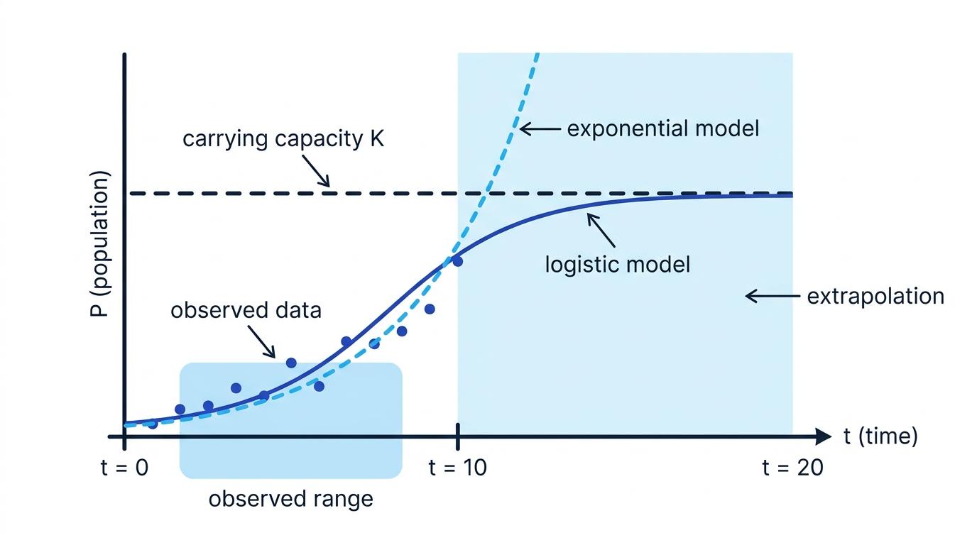
Graph comparing logistic and exponential population models, with observed data and an extrapolation region

Common Mistake

Long-range extrapolation

The further you extrapolate beyond the observed data, the more strongly your prediction depends on assumptions about the model's long-term behaviour.

Limitations of a model

Every model has limitations because it simplifies reality. Common limitations include:

assuming a constant rate when the rate may change;
ignoring external factors;
using measurements that contain random error;
assuming parameters remain fixed over time;
applying the model outside the interval where it was tested;
treating a continuous output as if it exactly represented a discrete quantity.

An exponential population model, for example, may assume unlimited food, space and other resources. This may be reasonable for a short time but unrealistic in the long term.

Common Mistake

Giving a vague limitation

Write a limitation that is specific to the context. Instead of saying “the model is inaccurate”, identify an assumption that may fail, such as “the model assumes that the percentage growth rate remains constant despite limited resources”.

Comparing predictions with data

A residual measures the difference between an observed value and the value predicted by a model.

Definition

Residual

For an observed value $y$ and predicted value $y^\hat y$ , the residual is

residual=y−y^.\text{residual}=y-\hat y.

A positive residual means the observed value is greater than the model's prediction. A negative residual means the model has overestimated the observed value.

Example

Calculating and interpreting a residual

A model predicts that sales in a particular month will be £42,500, but the observed sales are £40,900.

Calculate the residual using observed minus predicted:
$residual=40900−42500=−1600.\text{residual}=40900-42500=-1600.$
The residual is negative, so the observed sales were lower than the prediction.
Therefore, the model overestimated sales by £1600.

Small residuals with no clear pattern suggest that the model may be suitable. A systematic pattern suggests that the function is missing some important feature. For example, regularly alternating residuals might indicate seasonal behaviour.

Refining a model

To refine a model means to modify it so that it represents the real situation more accurately or is useful over a wider domain.

Possible refinements include:

changing the type of function;
adding another relevant variable;
allowing a parameter to vary with time;
restricting the model to a more suitable domain;
collecting more or better-quality data;
including periodic or seasonal effects;
replacing unrestricted exponential growth with a bounded model.

Example

Refining a population model

A fish population is modelled by $P(t)=200e^{0.3t}$ , but researchers know that the lake can support at most 5000 fish.

The exponential model is unsuitable in the long term because
$t→∞.P(t)\to\infty \quad \text{as } t\to\infty.$
This contradicts the known limit of 5000 fish.
A more appropriate model should still allow early growth but should approach 5000 rather than increasing without bound.
A logistic model such as
$P(t)=50001+Ae−kt,P(t)=\frac{5000}{1+Ae^{-kt}},$
where $A > 0$ and $k > 0$ , has the required limiting behaviour:
$t→∞.P(t)\to5000 \quad \text{as } t\to\infty.$
The parameters $A$ and $k$ could then be estimated using the observed population data.

Key Idea

Modelling is a cycle

A model is not simply chosen and accepted. You use it, compare its predictions with evidence, identify weaknesses and then refine it.

Exam technique

In the exam

Define variables clearly and include units where relevant.
Use every given condition to form equations for the model's parameters.
Check that your prediction lies in a sensible domain and interpret it in context.
Distinguish carefully between interpolation and extrapolation.
When discussing limitations or refinements, refer to a specific assumption and explain how the proposed change would improve the model.

Self review

Check yourself

How can you interpret the parameters in $y=Ae^{kt}$ ?
Why is extrapolation usually less reliable than interpolation?
How could you detect from residuals that a chosen function is unsuitable?

What you'll learn

How a function can represent a relationship between real-world quantities.
How to choose a suitable type of function and interpret its parameters.
How to test a model against data and use it to make predictions.
How to identify limitations and refine a model when it is not accurate enough.

From functions to models

You already know that a function maps each permitted input to exactly one output. It is often written as

y = f (x) .

In modelling, the input and output represent quantities from a real situation. For example, $t$ might represent time and $P (t)$ might represent the size of a population at time $t$ .

Definition

Mathematical model

A mathematical model is a simplified mathematical description of a real situation. A function model describes how one quantity depends on another.

A model is not the real situation itself. It deliberately ignores some details so that the main relationship can be analysed.