Revision notes for Edexcel AS Level Maths Statistical Distributions. Open each subtopic for explanations, worked examples, and summaries of Probability Distributions, The Binomial Distribution, and Cumulative Probabilities. Written against the Edexcel AS Level Maths (8MA0) specification, so the content matches what's examinable rather than general Maths background.
Statistical Distributions
What you'll learn
- How to describe a discrete random variable using a probability distribution.
- How to build and use a cumulative distribution function.
- How to recognise discrete uniform and binomial distributions.
- How to handle common exam-style tasks: missing probabilities, inequalities, independence, transformations, and expected counts.
1. Discrete random variables and probability distributions
A random variable is a variable whose value depends on chance.
A random variable is discrete if it can only take separate, countable values, such as 0, 1, 2, 3 or the score on a spinner.
Definition
Discrete probability distribution
A discrete probability distribution lists every possible value of a random variable and the probability of each value. The probabilities must:
- each be between 0 and 1
- add up to 1
For example, if XXX is the number scored on a spinner, then P(X=x)P(X=x)P(X=x) means “the probability that XXX takes the value xxx”.
Key Idea
The total probability rule
For any complete probability distribution:
∑P(X=x)=1\sum P(X=x)=1∑P(X=x)=1This is usually the quickest way to find a missing constant.
Worked example: finding a missing probability
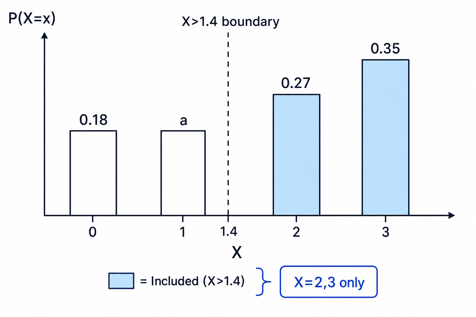
A discrete random variable XXX has this probability distribution:
| Value of X | 0 | 1 | 2 | 3 |
|---|---|---|---|---|
| Probability | 0.18 | a | 0.27 | 0.35 |
Find the value of aaa, then find P(X>1.4)P(X>1.4)P(X>1.4).
Example
Missing value and an inequality
-
Use the fact that all probabilities add to 1:
0.18+a+0.27+0.35=10.18+a+0.27+0.35=10.18+a+0.27+0.35=1 -
Solve for aaa:
a=1−0.18−0.27−0.35=0.20a=1-0.18-0.27-0.35=0.20a=1−0.18−0.27−0.35=0.20 -
Interpret the inequality carefully. Since XXX can only be 0, 1, 2 or 3, the values greater than 1.4 are 2 and 3.
-
Add the relevant probabilities:
P(X>1.4)=P(X=2)+P(X=3)=0.27+0.35=0.62P(X>1.4)=P(X=2)+P(X=3)=0.27+0.35=0.62P(X>1.4)=P(X=2)+P(X=3)=0.27+0.35=0.62
Common Mistake
Treating a discrete variable as continuous
If XXX only takes integer values, then P(X>1.4)P(X>1.4)P(X>1.4) is the same as P(X≥2)P(X\ge 2)P(X≥2). Do not try to include “part” of the probability at 1 or 2.
2. Cumulative distribution functions
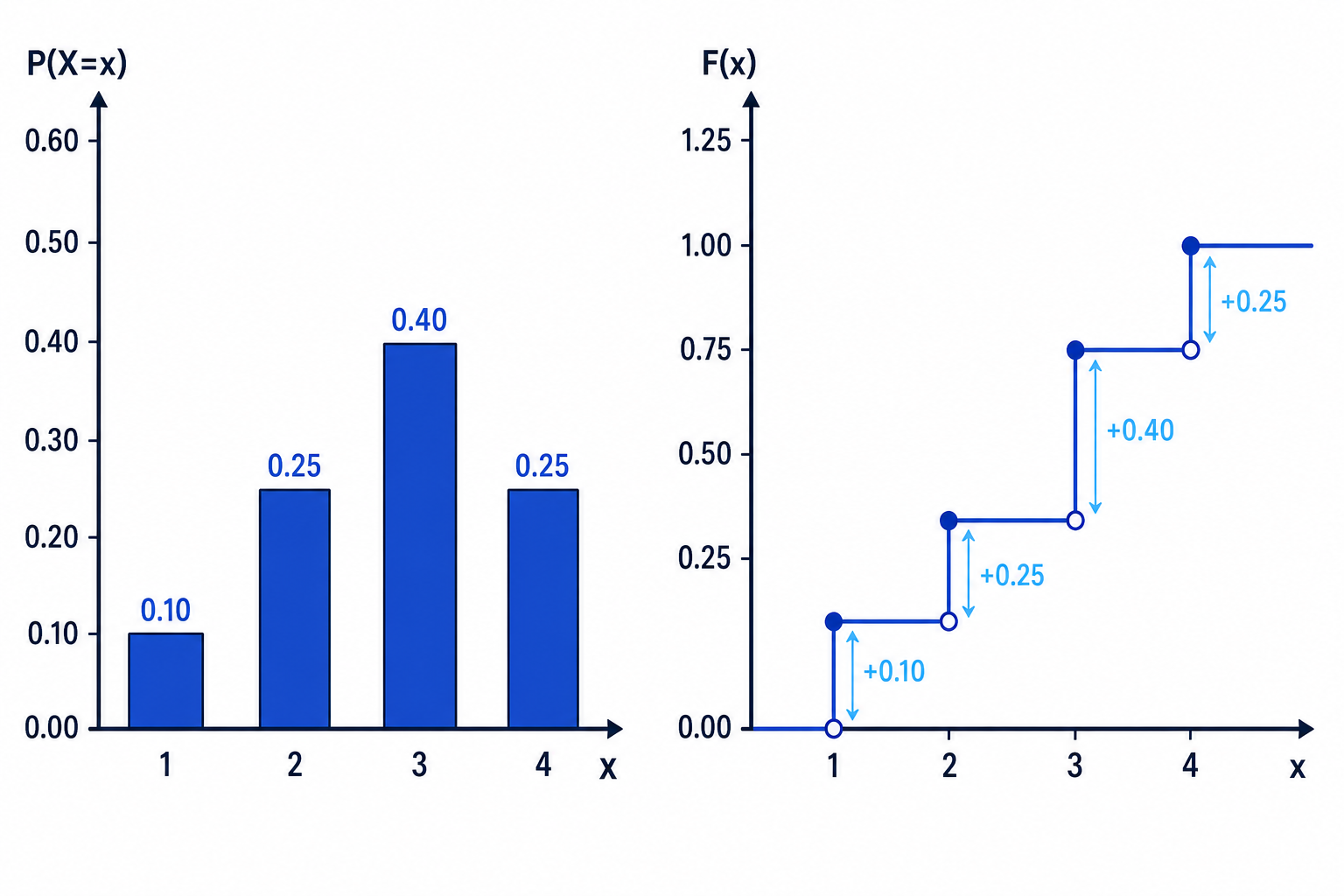
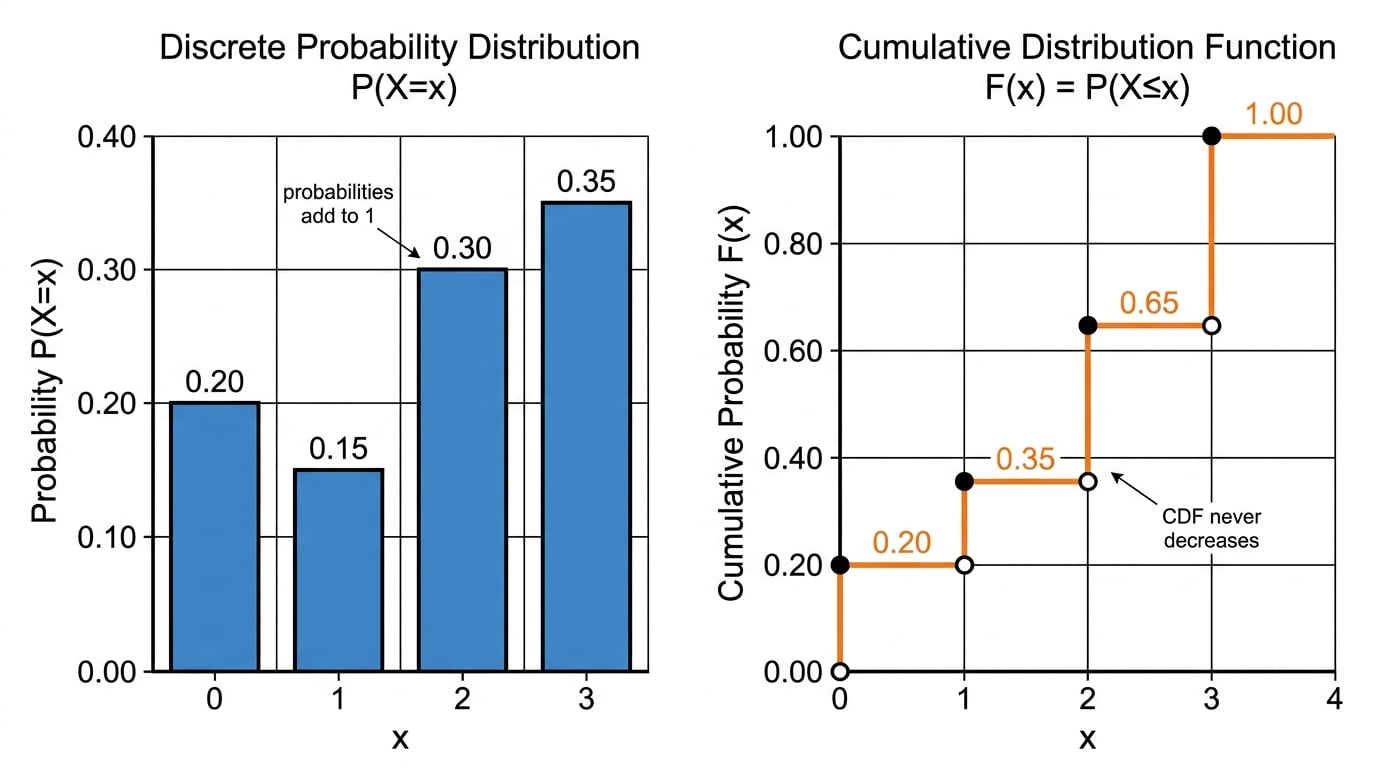
The cumulative distribution function, often written as F(x)F(x)F(x), gives the probability that the random variable is less than or equal to a value.
Definition
Cumulative distribution function
For a random variable XXX,
F(x)=P(X≤x)F(x)=P(X\le x)F(x)=P(X≤x)So F(x)F(x)F(x) is the running total of probabilities up to and including xxx.
A cumulative distribution for a discrete variable increases in jumps, because probability is only added at the possible values of XXX.
Worked example: constructing a cumulative table
A random variable XXX has the distribution below.
| Value of X | 1 | 2 | 3 | 4 |
|---|---|---|---|---|
| Probability | 0.10 | 0.25 | 0.40 | 0.25 |
Construct a table for F(x)F(x)F(x).
Example
Building the cumulative distribution
-
Start with the first value:
F(1)=P(X≤1)=0.10F(1)=P(X\le 1)=0.10F(1)=P(X≤1)=0.10 -
Add the probability at 2:
F(2)=P(X≤2)=0.10+0.25=0.35F(2)=P(X\le 2)=0.10+0.25=0.35F(2)=P(X≤2)=0.10+0.25=0.35 -
Add the probability at 3:
F(3)=P(X≤3)=0.10+0.25+0.40=0.75F(3)=P(X\le 3)=0.10+0.25+0.40=0.75F(3)=P(X≤3)=0.10+0.25+0.40=0.75 -
Add the probability at 4:
F(4)=1F(4)=1F(4)=1 -
Write the cumulative table:
| Value of X | 1 | 2 | 3 | 4 |
|---|---|---|---|---|
| Cumulative probability | 0.10 | 0.35 | 0.75 | 1.00 |
Tip
CDF sanity checks
A cumulative distribution should never go down, and the final value should be 1.
3. Discrete uniform distributions
A discrete uniform distribution occurs when each possible outcome is equally likely.
Definition
Discrete uniform distribution
If a random variable has nnn equally likely values, then each value has probability 1n\frac{1}{n}n1.
Common examples include a fair die, a fair spinner with equal sectors, or choosing one card from equally likely labelled cards.
Worked example: fair spinner
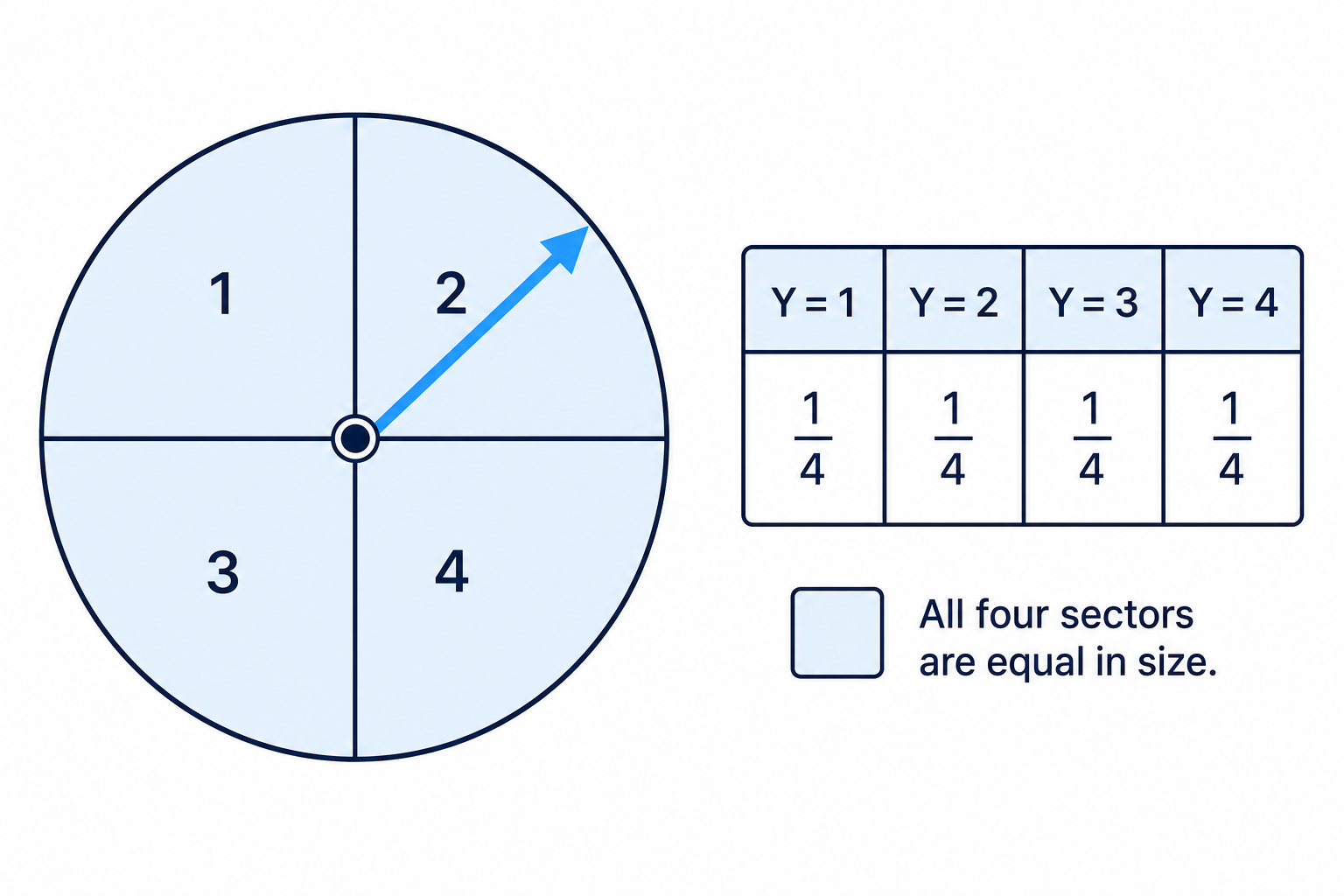
A fair spinner has four equal sectors labelled 1, 2, 3 and 4. Let YYY be the number landed on.
Example
Writing down a uniform distribution
-
Since the spinner is fair, all four outcomes are equally likely.
-
There are four possible values, so each probability is:
14\frac{1}{4}41 -
The probability distribution is:
| Value of Y | 1 | 2 | 3 | 4 |
|---|---|---|---|---|
| Probability | 1/4 | 1/4 | 1/4 | 1/4 |
- The name of the distribution is the discrete uniform distribution.
4. The binomial distribution
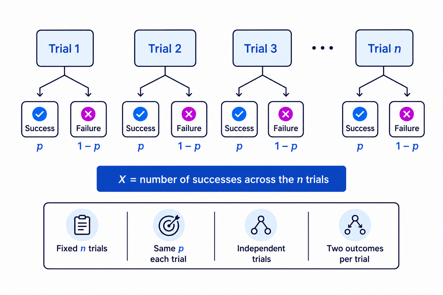
The binomial distribution models the number of successes in a fixed number of repeated trials.
Definition
Binomial distribution
We write X∼B(n,p)X\sim B(n,p)X∼B(n,p) when:
- there are nnn trials
- each trial has two outcomes: success or failure
- the probability of success is constant, ppp
- the trials are independent
- XXX counts the number of successes
The formula for exactly rrr successes is:
P(X=r)=(nr)pr(1−p)n−rP(X=r)=\binom{n}{r}p^r(1-p)^{n-r}P(X=r)=(rn)pr(1−p)n−rHere, (nr)\binom{n}{r}(rn) counts how many different ways the successes can be arranged.
Worked example: exactly, less than, and at least
A student has probability 0.3 of answering a question correctly. They answer 12 independent questions. Let XXX be the number answered correctly.
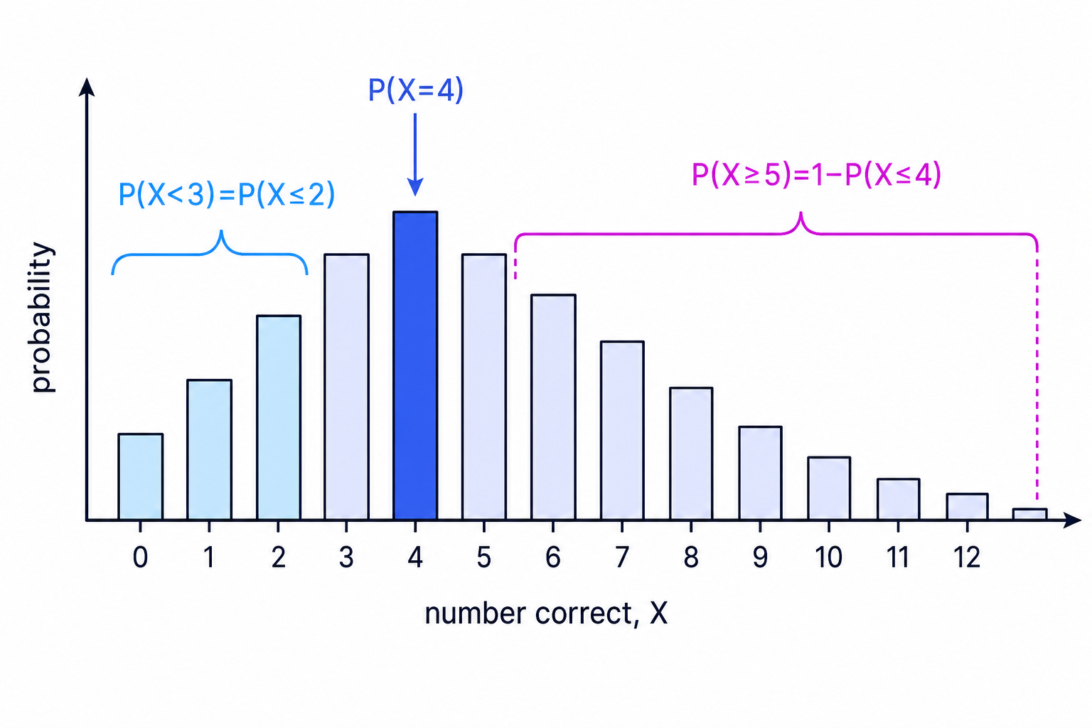
Find P(X=4)P(X=4)P(X=4), P(X<3)P(X<3)P(X<3), and P(X≥5)P(X\ge 5)P(X≥5).
Example
Using a binomial model
-
Identify the distribution:
X∼B(12,0.3)X\sim B(12,0.3)X∼B(12,0.3) -
For exactly 4 correct answers, use the binomial formula:
P(X=4)=(124)(0.3)4(0.7)8P(X=4)=\binom{12}{4}(0.3)^4(0.7)^8P(X=4)=(412)(0.3)4(0.7)8 -
Evaluate:
P(X=4)≈0.231P(X=4)\approx 0.231P(X=4)≈0.231 -
For P(X<3)P(X<3)P(X<3), include 0, 1 and 2:
P(X<3)=P(X≤2)P(X<3)=P(X\le 2)P(X<3)=P(X≤2) -
Using a calculator’s binomial cumulative function, or by adding the three terms:
P(X≤2)≈0.253P(X\le 2)\approx 0.253P(X≤2)≈0.253 -
For P(X≥5)P(X\ge 5)P(X≥5), use the complement:
P(X≥5)=1−P(X≤4)P(X\ge 5)=1-P(X\le 4)P(X≥5)=1−P(X≤4) -
Evaluate:
P(X≥5)≈1−0.7237=0.276P(X\ge 5)\approx 1-0.7237=0.276P(X≥5)≈1−0.7237=0.276
Common Mistake
Wrong boundary in binomial inequalities
For integer-valued XXX, P(X<3)P(X<3)P(X<3) means P(X≤2)P(X\le 2)P(X≤2), not P(X≤3)P(X\le 3)P(X≤3). Similarly, P(X>4)P(X>4)P(X>4) means P(X≥5)P(X\ge 5)P(X≥5).
5. Checking binomial assumptions
Before using a binomial model, check that the situation really matches the conditions.
For example, “number of hits in 8 darts” can be binomial if each throw has the same probability of a hit and throws are independent.
But “number of goals in a football match” might be less realistic as binomial, because scoring chances are not necessarily independent and the probability of scoring may change during the match.
Worked example: modelling hits
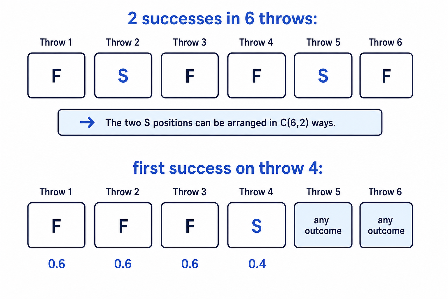
A player throws 6 balls at a bucket. The probability of a successful throw is 0.4. Assume throws are independent.
Let XXX be the number of successful throws.
Find P(X=2)P(X=2)P(X=2). Then find the probability that the first success is on the fourth throw.
Example
Binomial probability and first success
-
For the number of successes in 6 throws:
X∼B(6,0.4)X\sim B(6,0.4)X∼B(6,0.4) -
Find exactly 2 successes:
P(X=2)=(62)(0.4)2(0.6)4P(X=2)=\binom{6}{2}(0.4)^2(0.6)^4P(X=2)=(26)(0.4)2(0.6)4 -
Evaluate:
P(X=2)≈0.311P(X=2)\approx 0.311P(X=2)≈0.311 -
For the first success on the fourth throw, the first three throws must be failures and the fourth must be a success.
-
Multiply the probabilities:
P(first success on throw 4)=(0.6)3(0.4)=0.0864P(\text{first success on throw }4)=(0.6)^3(0.4)=0.0864P(first success on throw 4)=(0.6)3(0.4)=0.0864
Common Mistake
First success is not the same as exactly one success
“First success on throw 4” says what happens on throws 1 to 4 only: fail, fail, fail, success. It does not automatically describe later throws unless the question says so.
6. Expected counts from a probability
If an event has probability ppp and it is repeated across NNN independent occasions, the expected number of occasions on which it happens is:
NpNpNpThis is useful when a binomial model is used inside a larger context.
Worked example: expected number of matches
A team’s number of goals in a match is modelled by X∼B(9,0.2)X\sim B(9,0.2)X∼B(9,0.2).
Using this model, find the expected number of matches with no goals in a 30-match season.
Example
Expected number using a model
-
First find the probability of no goals in one match:
P(X=0)=(90)(0.2)0(0.8)9P(X=0)=\binom{9}{0}(0.2)^0(0.8)^9P(X=0)=(09)(0.2)0(0.8)9 -
Simplify:
P(X=0)=(0.8)9≈0.134P(X=0)=(0.8)^9\approx 0.134P(X=0)=(0.8)9≈0.134 -
Multiply by the number of matches:
30×0.134≈4.0330\times 0.134\approx 4.0330×0.134≈4.03 -
So the expected number of goalless matches is about 4.
Tip
Interpreting expected values
An expected number does not have to be a whole number. It is a long-run average, not a guaranteed outcome.
7. Combining independent random variables
Sometimes a question involves two independent attempts, games, or random variables.
If two events are independent, the result of one does not affect the result of the other. For independent events, you multiply probabilities.
Worked example: total score from two games
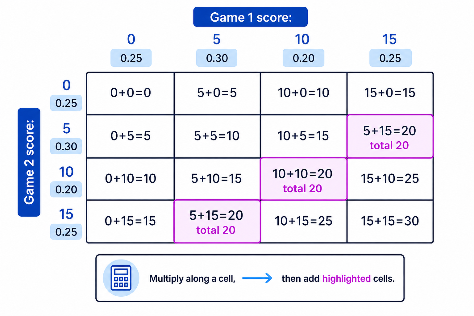
In one game, a player can score 0, 5, 10 or 15 points with probabilities:
| Score | 0 | 5 | 10 | 15 |
|---|---|---|---|---|
| Probability | 0.25 | 0.30 | 0.20 | 0.25 |
The player plays twice independently. Find the probability that the total score is 20.
Example
Adding scores from independent games
-
List the score pairs that total 20:
(5,15), (10,10), (15,5)(5,15),\ (10,10),\ (15,5)(5,15), (10,10), (15,5) -
Multiply probabilities within each pair because the games are independent:
P(5,15)=0.30×0.25P(5,15)=0.30\times 0.25P(5,15)=0.30×0.25 -
Do the same for all possible pairs and add them:
P(total 20)=(0.30)(0.25)+(0.20)(0.20)+(0.25)(0.30)P(\text{total }20)=(0.30)(0.25)+(0.20)(0.20)+(0.25)(0.30)P(total 20)=(0.30)(0.25)+(0.20)(0.20)+(0.25)(0.30) -
Evaluate:
P(total 20)=0.075+0.040+0.075=0.190P(\text{total }20)=0.075+0.040+0.075=0.190P(total 20)=0.075+0.040+0.075=0.190
8. Transforming a random variable
A transformed random variable is made from another random variable using a formula, such as Y=7−2XY=7-2XY=7−2X.
To find probabilities involving YYY, replace YYY with its formula and solve the inequality for XXX.
Worked example: using a transformation
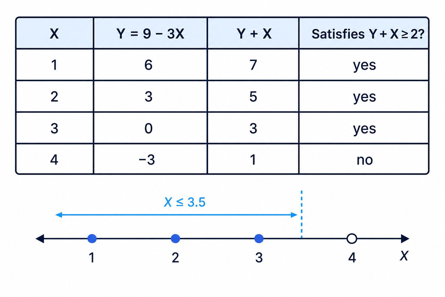
Let XXX take the values 1, 2, 3 and 4. Suppose Y=9−3XY=9-3XY=9−3X. Find P(Y+X≥2)P(Y+X\ge 2)P(Y+X≥2).
Example
Rewriting the inequality in terms of X
-
Substitute Y=9−3XY=9-3XY=9−3X into the inequality:
Y+X≥2Y+X\ge 2Y+X≥2 -
Simplify in terms of XXX:
9−3X+X≥29-3X+X\ge 29−3X+X≥2 -
Solve:
9−2X≥29-2X\ge 29−2X≥2 -
Continue solving:
−2X≥−7-2X\ge -7−2X≥−7 -
Divide by a negative number, remembering to reverse the inequality:
X≤3.5X\le 3.5X≤3.5 -
Since XXX can only be 1, 2, 3 or 4, this means X=1,2,3X=1,2,3X=1,2,3.
-
Add the relevant probabilities from the distribution of XXX.
Common Mistake
Forgetting to reverse the inequality
When you divide an inequality by a negative number, the inequality sign changes direction.
Exam technique
In the exam
-
Check whether the variable is discrete: inequalities usually need careful conversion, such as X<4X<4X<4 becoming X≤3X\le 3X≤3.
-
For a probability table, always use “probabilities add to 1” first if a constant is missing.
-
For binomial questions, write X∼B(n,p)X\sim B(n,p)X∼B(n,p) before calculating so you are clear about the number of trials and success probability.
-
Use complements for phrases like “more than”, “at least”, and “at least one” when it saves time.
-
When combining independent events, multiply along a specific route and add different possible routes.
Self review
Check yourself
-
Can you explain the difference between P(X=x)P(X=x)P(X=x) and F(x)F(x)F(x)?
-
If X∼B(20,0.15)X\sim B(20,0.15)X∼B(20,0.15), what values of nnn and ppp are being used?
-
For a discrete random variable, why is P(X<6)P(X<6)P(X<6) usually rewritten as P(X≤5)P(X\le 5)P(X≤5)?

Recap questions
Test yourself with 5 quick questions on this guide. Answer them all correctly to complete it.
You've reached the end
Test yourself on this topic, or move on to the next guide.
How was this guide?