Revision notes for Edexcel AS Level Maths Differentiation. Open each subtopic for explanations, worked examples, and summaries of 12.1 Gradients of Curves, 12.2 Differentiation from first principles, 12.3 Differentiating x^n, 12.4 Differentiating Quadratics, 12.5 Differentiating functions with two or more terms, 12.6 Gradients, Tangents and Normals, 12.7 Increasing and Decreasing Functions, 12.8 Second Order Derivatives, 12.9 Stationary Points, 12.10 Sketching Gradient Functions, and 12.11 Modelling with Differentiation. Written against the Edexcel AS Level Maths (8MA0) specification, so the content matches what's examinable rather than general Maths background.
Differentiation
What you'll learn
- What dydx\frac{dy}{dx}dxdy and f′(x)f'(x)f′(x) mean.
- How to differentiate powers of xxx, including roots and fractions.
- How to find gradients, tangents, normals and stationary points.
- How differentiation helps solve maximum and minimum problems.
1. Gradient and the derivative
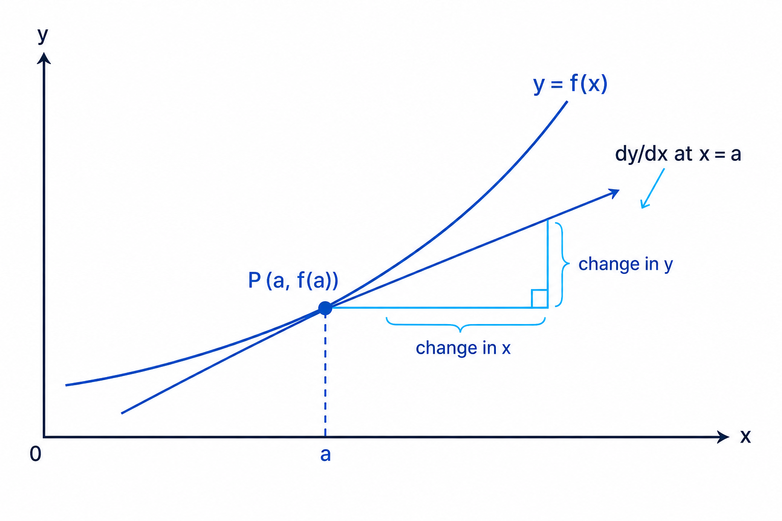
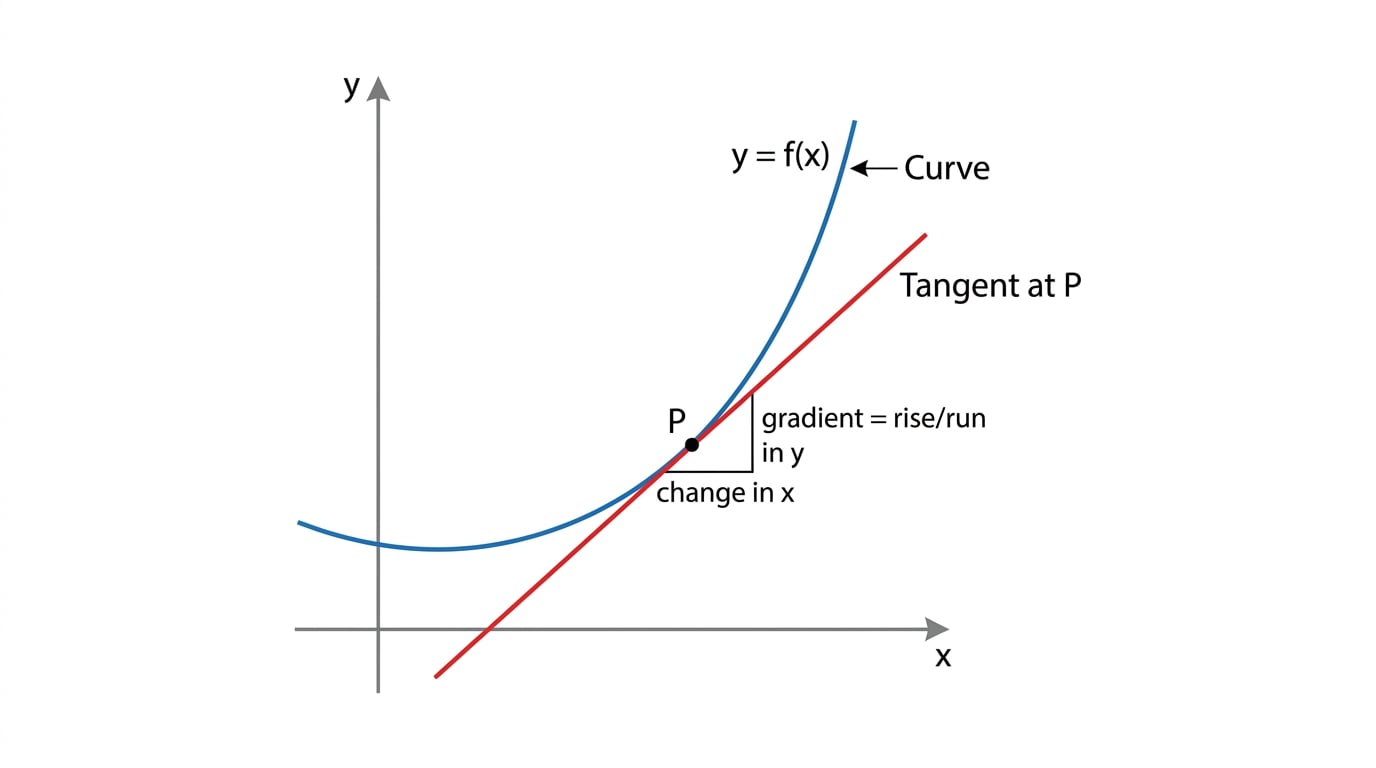
You already know that the gradient of a straight line is “change in yyy divided by change in xxx”. A curve is different: its gradient can change from point to point.
To find the gradient of a curve at one point, we use the tangent there: the straight line that touches the curve and has the same gradient at that point.
Definition
Derivative
The derivative of yyy with respect to xxx, written dydx\frac{dy}{dx}dxdy, is the function that gives the gradient of the curve at each value of xxx. If the function is called f(x)f(x)f(x), its derivative can also be written as f′(x)f'(x)f′(x).
To differentiate means “find the derivative”.
2. The power rule
Most AS differentiation questions begin with expressions made from powers of xxx, such as x3x^3x3, x2x^2x2 or x−1x^{-1}x−1.
A coefficient is the number multiplying a power of xxx. For example, in 5x35x^35x3, the coefficient is 5.
Key Idea
The power rule
For any constant coefficient aaa and power nnn,
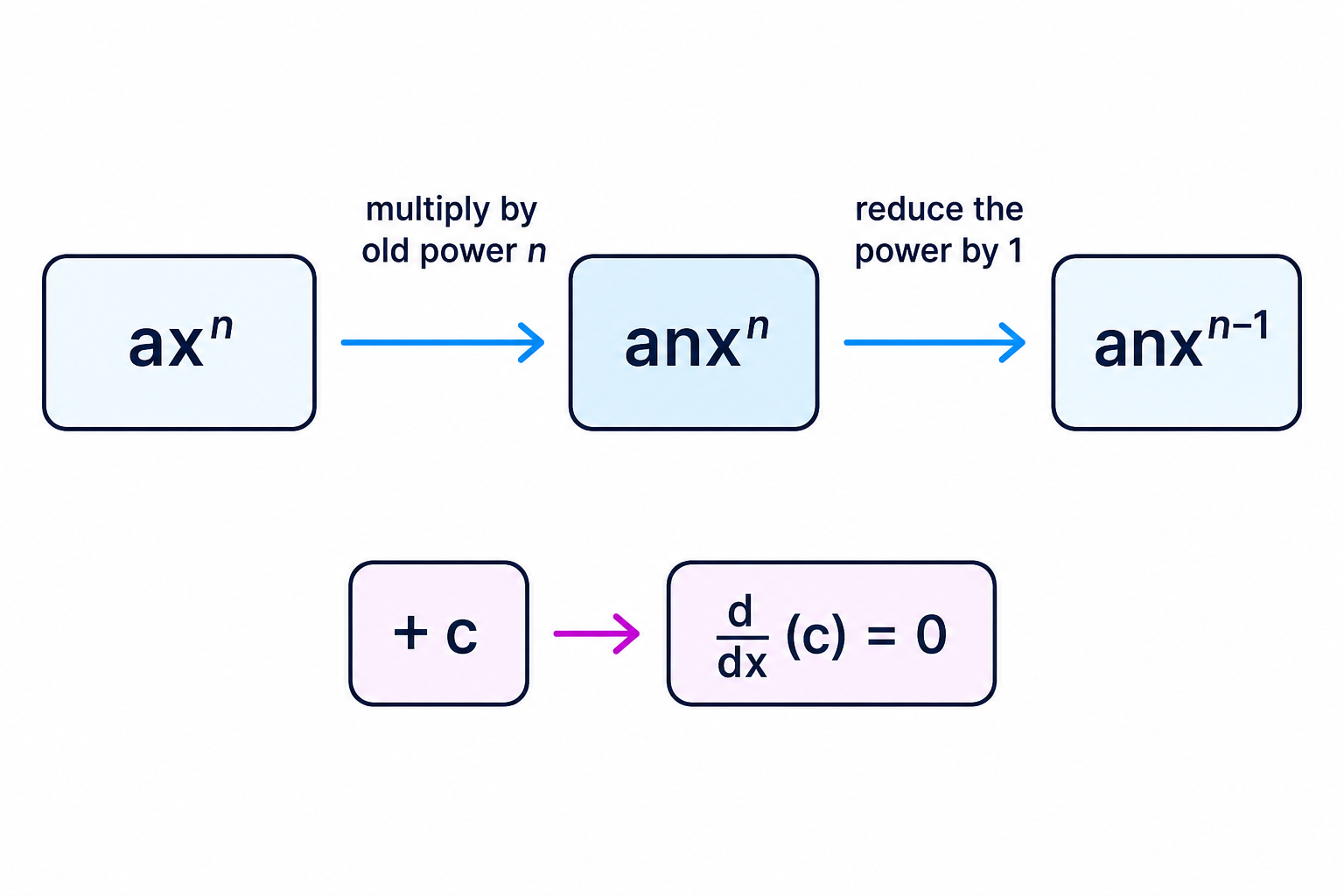
ddx(axn)=anxn−1\frac{d}{dx}(ax^n)=anx^{n-1}dxd(axn)=anxn−1A constant on its own differentiates to 0.
So you multiply by the old power, then reduce the power by 1.
Example
Differentiate a polynomial and find a gradient
For y=3x3−4x2+6x−8y=3x^3-4x^2+6x-8y=3x3−4x2+6x−8, find dydx\frac{dy}{dx}dxdy and the gradient when x=2x=2x=2.
-
Differentiate each term using the power rule.
dydx=9x2−8x+6\frac{dy}{dx}=9x^2-8x+6dxdy=9x2−8x+6 -
Substitute x=2x=2x=2 into the derivative.
9(2)2−8(2)+6=269(2)^2-8(2)+6=269(2)2−8(2)+6=26 -
The gradient of the curve when x=2x=2x=2 is 26.
Common Mistake
Substituting too early
Differentiate first, then put in the given xxx-value. If you put x=2x=2x=2 into yyy first, you only get a coordinate, not a gradient.
3. Rewriting roots and fractions
The power rule works beautifully if everything is written as a power of xxx.
Useful rewrites are:
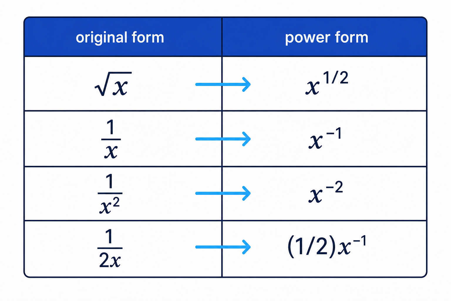
- x=x1/2\sqrt{x}=x^{1/2}x=x1/2
- 1x=x−1\frac{1}{x}=x^{-1}x1=x−1
- 1x2=x−2\frac{1}{x^2}=x^{-2}x21=x−2
- 12x=12x−1\frac{1}{2x}=\frac{1}{2}x^{-1}2x1=21x−1
This is why simplifying algebra before differentiating is often the main skill.
Definition
Second derivative
The second derivative, written d2ydx2\frac{d^2y}{dx^2}dx2d2y, is found by differentiating dydx\frac{dy}{dx}dxdy. It tells you how the gradient is changing.
Example
Differentiate roots and fractions
For y=6x+4x+7y=6\sqrt{x}+\frac{4}{x}+7y=6x+x4+7, find dydx\frac{dy}{dx}dxdy and d2ydx2\frac{d^2y}{dx^2}dx2d2y.
-
Rewrite the root and fraction as powers.
y=6x1/2+4x−1+7y=6x^{1/2}+4x^{-1}+7y=6x1/2+4x−1+7 -
Differentiate once.
dydx=3x−1/2−4x−2\frac{dy}{dx}=3x^{-1/2}-4x^{-2}dxdy=3x−1/2−4x−2 -
Differentiate again.
d2ydx2=−32x−3/2+8x−3\frac{d^2y}{dx^2}=-\frac{3}{2}x^{-3/2}+8x^{-3}dx2d2y=−23x−3/2+8x−3
Tip
Answer form
Negative powers are usually acceptable unless the question asks for a particular form. If you want, x−2x^{-2}x−2 can be rewritten as 1x2\frac{1}{x^2}x21.
4. Stationary points, increasing and decreasing
The sign of dydx\frac{dy}{dx}dxdy tells you what the curve is doing.
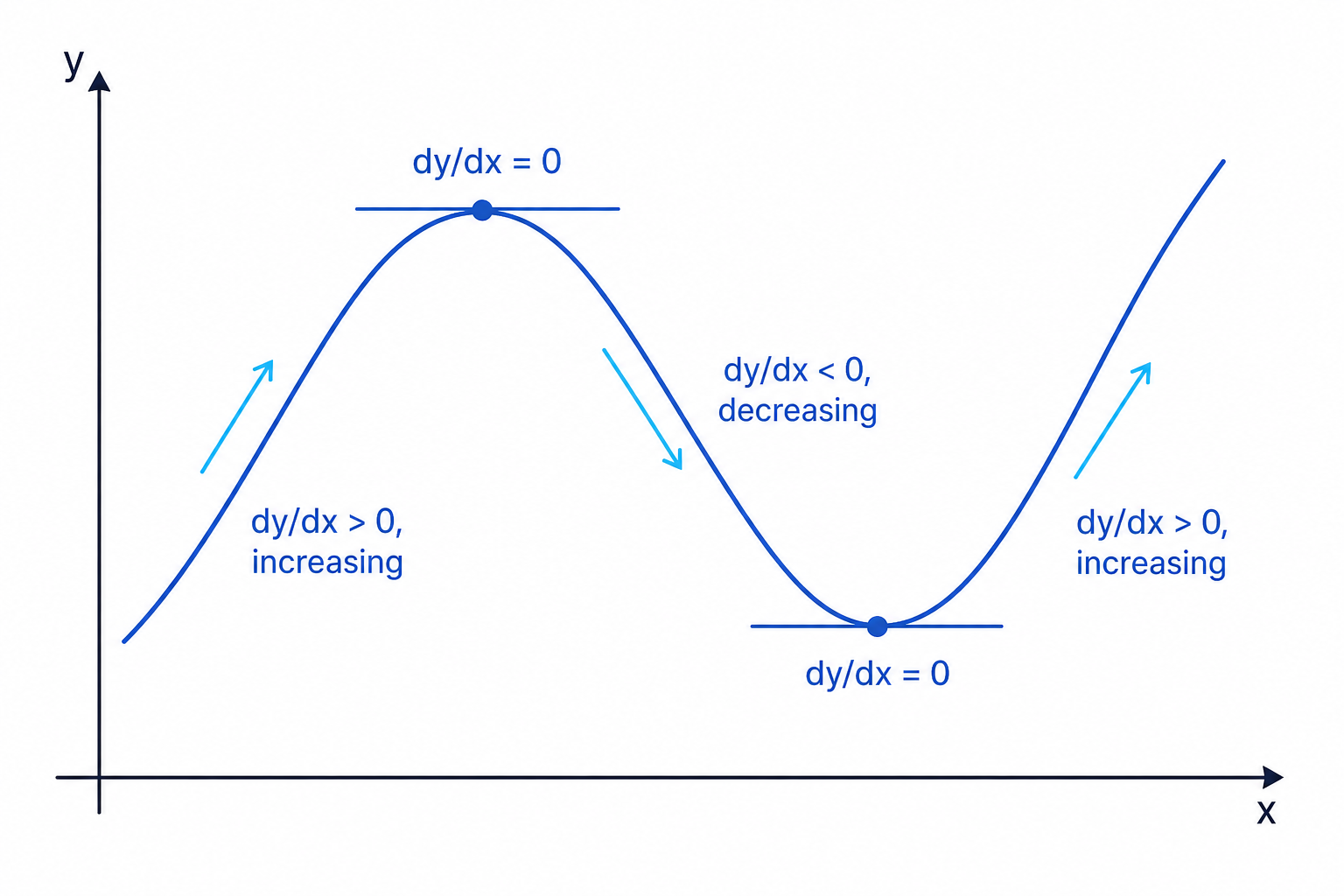
- If dydx>0\frac{dy}{dx}>0dxdy>0, the curve is increasing.
- If dydx<0\frac{dy}{dx}<0dxdy<0, the curve is decreasing.
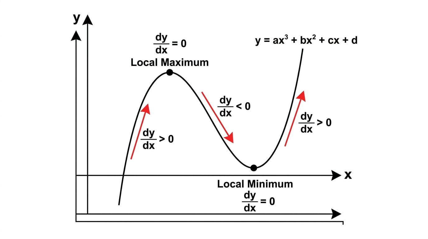
- If dydx=0\frac{dy}{dx}=0dxdy=0, the curve has a stationary point.
Definition
Stationary points
-
A stationary point is a point on a curve where the gradient is zero.
-
A local maximum is a high point compared with nearby points.
-
A local minimum is a low point compared with nearby points.
The second derivative can help classify stationary points:
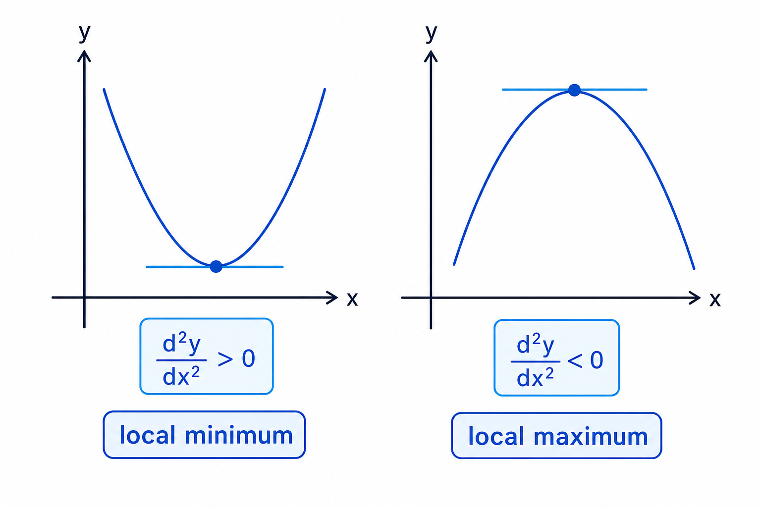
- If d2ydx2>0\frac{d^2y}{dx^2}>0dx2d2y>0, the point is a local minimum.
- If d2ydx2<0\frac{d^2y}{dx^2}<0dx2d2y<0, the point is a local maximum.
Example
Find and classify stationary points
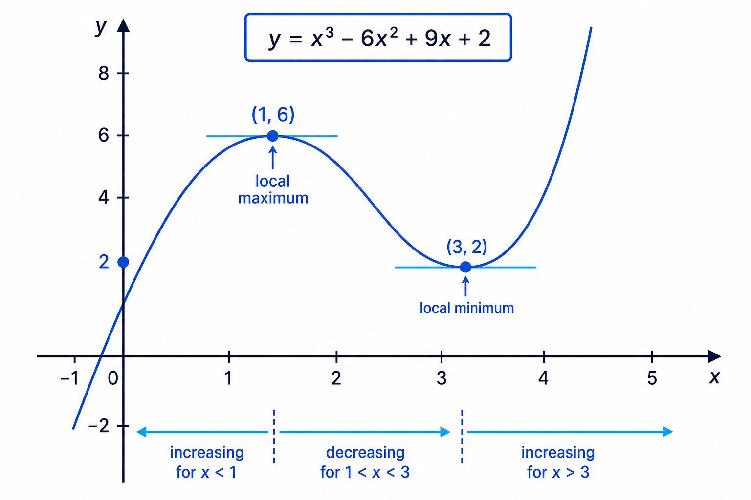
For y=x3−6x2+9x+2y=x^3-6x^2+9x+2y=x3−6x2+9x+2, find the stationary points and determine their nature.
-
Differentiate.
dydx=3x2−12x+9=3(x−1)(x−3)\frac{dy}{dx}=3x^2-12x+9=3(x-1)(x-3)dxdy=3x2−12x+9=3(x−1)(x−3) -
Set the derivative equal to zero.
3(x−1)(x−3)=0⇒x=1 or x=33(x-1)(x-3)=0 \Rightarrow x=1 \text{ or } x=33(x−1)(x−3)=0⇒x=1 or x=3 -
Find the corresponding yyy-coordinates.
y(1)=1−6+9+2=6y(3)=27−54+27+2=2\begin{aligned} y(1)&=1-6+9+2=6\\ y(3)&=27-54+27+2=2 \end{aligned}y(1)y(3)=1−6+9+2=6=27−54+27+2=2 -
Use the second derivative to classify the points.
d2ydx2=6x−12x=1:6(1)−12=−6<0⇒local maximumx=3:6(3)−12=6>0⇒local minimum\begin{aligned} \frac{d^2y}{dx^2}&=6x-12\\ x=1 &: 6(1)-12=-6<0 \Rightarrow \text{local maximum}\\ x=3 &: 6(3)-12=6>0 \Rightarrow \text{local minimum} \end{aligned}dx2d2yx=1x=3=6x−12:6(1)−12=−6<0⇒local maximum:6(3)−12=6>0⇒local minimum -
The curve has a local maximum at (1,6)(1,6)(1,6) and a local minimum at (3,2)(3,2)(3,2).
-
Use the sign of 3(x−1)(x−3)3(x-1)(x-3)3(x−1)(x−3) to find where the curve is increasing or decreasing.
increasing: x<1 or x>3decreasing: 1<x<3\begin{aligned} \text{increasing: }&x<1 \text{ or } x>3\\ \text{decreasing: }&1<x<3 \end{aligned}increasing: decreasing: x<1 or x>31<x<3
Common Mistake
Stationary does not always mean maximum
Solving dydx=0\frac{dy}{dx}=0dxdy=0 only finds possible maximum or minimum points. You still need to classify them using the second derivative or a sign-change test.
5. Tangents and normals
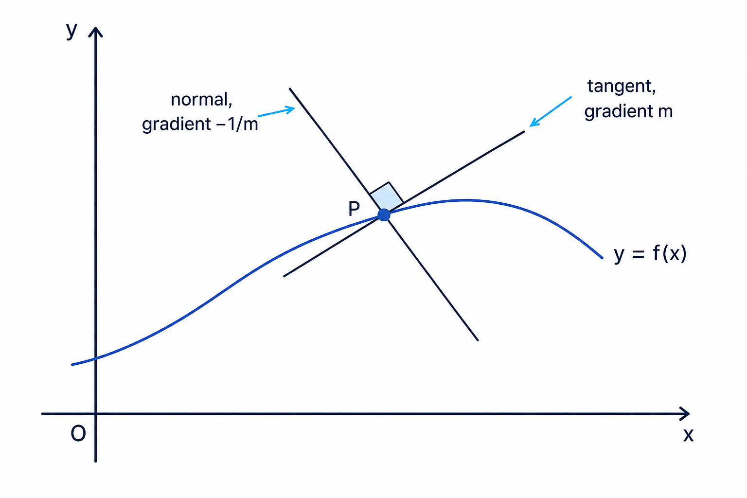
A tangent uses the gradient of the curve at a point. A normal is perpendicular to the tangent.
Definition
Tangent and normal
-
A tangent is a straight line with the same gradient as the curve at a point.
-
A normal is a straight line perpendicular to the tangent at that point.
For a line through (a,b)(a,b)(a,b) with gradient mmm, use:
y−b=m(x−a)y-b=m(x-a)y−b=m(x−a)Then rearrange into the form requested, such as y=mx+cy=mx+cy=mx+c or ax+by+c=0ax+by+c=0ax+by+c=0.
If the tangent gradient is mmm, the normal gradient is −1m-\frac{1}{m}−m1.
Common Mistake
Horizontal tangents
If the tangent gradient is 0, the normal is vertical, so its equation is of the form x=ax=ax=a. The formula −1m-\frac{1}{m}−m1 would involve division by zero.
Example
Find the equation of a normal
For y=(2x+1)(x−3)xy=\frac{(2x+1)(x-3)}{x}y=x(2x+1)(x−3), find the equation of the normal when x=−1x=-1x=−1, giving your answer in the form ax+by+c=0ax+by+c=0ax+by+c=0.
-
Expand and divide by xxx first.
y=2x2−5x−3x=2x−5−3x−1y=\frac{2x^2-5x-3}{x}=2x-5-3x^{-1}y=x2x2−5x−3=2x−5−3x−1 -
Differentiate, then evaluate the tangent gradient at x=−1x=-1x=−1.
dydx=2+3x−2,mtangent=2+3(−1)−2=5\frac{dy}{dx}=2+3x^{-2},\qquad m_{\text{tangent}}=2+3(-1)^{-2}=5dxdy=2+3x−2,mtangent=2+3(−1)−2=5 -
Find the point on the curve.
y(−1)=2(−1)−5−3(−1)−1=−4y(-1)=2(-1)-5-3(-1)^{-1}=-4y(−1)=2(−1)−5−3(−1)−1=−4 -
Find the normal gradient.
mnormal=−15m_{\text{normal}}=-\frac{1}{5}mnormal=−51 -
Use the point-gradient form through (−1,−4)(-1,-4)(−1,−4).
y+4=−15(x+1)y+4=-\frac{1}{5}(x+1)y+4=−51(x+1) -
Rearrange into integer form.
x+5y+21=0x+5y+21=0x+5y+21=0
6. Optimisation
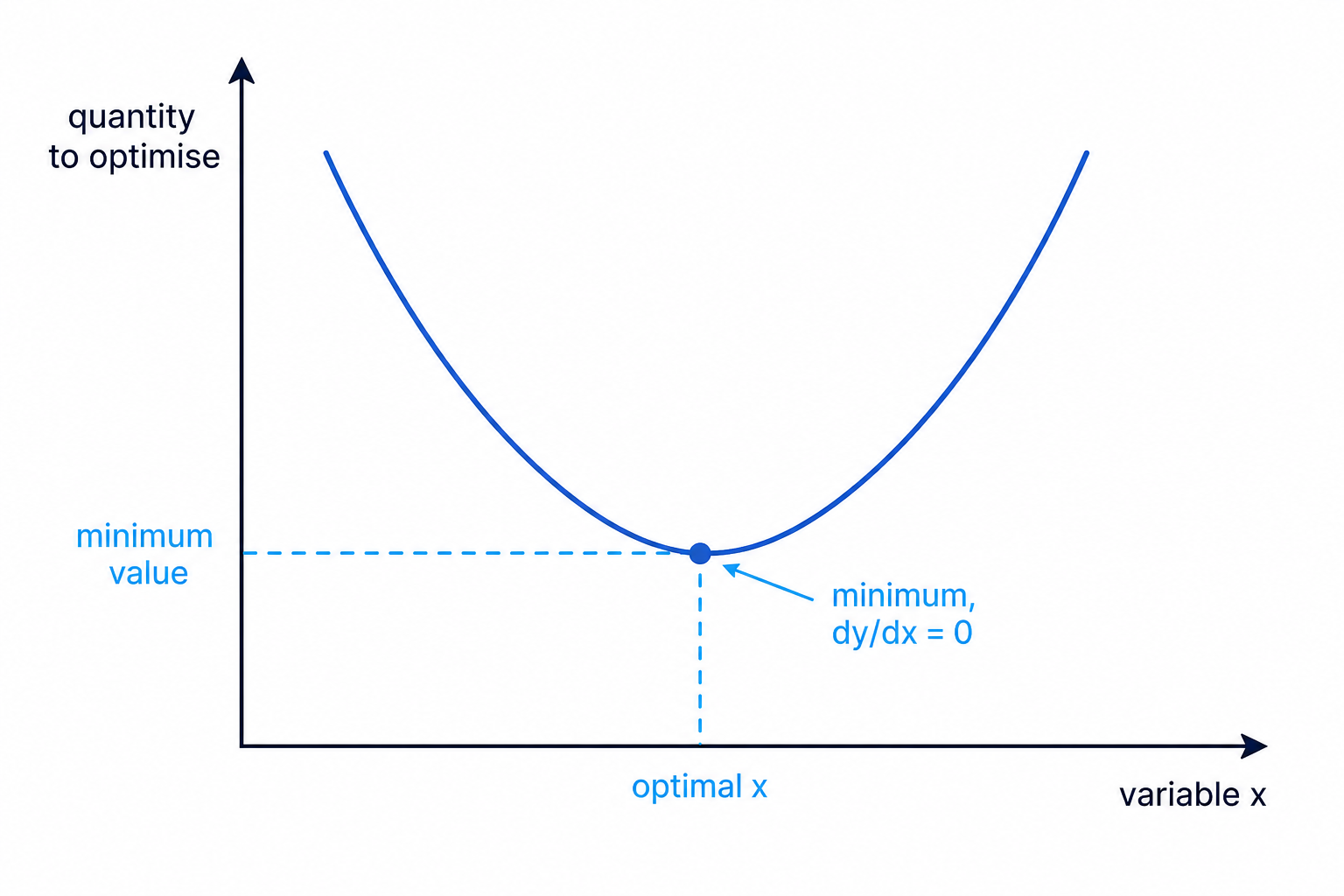
Optimisation means finding the value that makes something as large or as small as possible. In differentiation, this usually means finding a maximum or minimum.
Key Idea
Optimisation recipe
-
Write the quantity to be optimised as a function of one variable.
-
Differentiate.
-
Set the derivative equal to zero and solve.
-
Use the second derivative, or another argument, to justify maximum or minimum.
-
Substitute back to find the required value.
Example
Minimising a cost model
A journey has cost CCC pounds when driven at speed vvv mph, where
C=3200v+2v+15C=\frac{3200}{v}+2v+15C=v3200+2v+15Find the speed that minimises the cost, and find the minimum cost.
-
Rewrite using powers of vvv.
C=3200v−1+2v+15C=3200v^{-1}+2v+15C=3200v−1+2v+15 -
Differentiate.
dCdv=−3200v−2+2\frac{dC}{dv}=-3200v^{-2}+2dvdC=−3200v−2+2 -
Solve dCdv=0\frac{dC}{dv}=0dvdC=0. Since v>0v>0v>0, keep the positive root.
−3200v2+2=0⇒2v2=3200⇒v2=1600⇒v=40-\frac{3200}{v^2}+2=0 \Rightarrow 2v^2=3200 \Rightarrow v^2=1600 \Rightarrow v=40−v23200+2=0⇒2v2=3200⇒v2=1600⇒v=40 -
Check using the second derivative.
d2Cdv2=6400v−3when v=40,d2Cdv2>0\begin{aligned} \frac{d^2C}{dv^2}&=6400v^{-3}\\ \text{when }v=40,\quad \frac{d^2C}{dv^2}&>0 \end{aligned}dv2d2Cwhen v=40,dv2d2C=6400v−3>0 -
Calculate the minimum cost.
C=320040+2(40)+15=175C=\frac{3200}{40}+2(40)+15=175C=403200+2(40)+15=175 -
The minimum cost is £175, achieved at 40 mph.
Tip
When a model has two variables
Use the given constraint, such as a fixed surface area, to rewrite the quantity in one variable before differentiating. You cannot optimise a formula with two changing variables using ordinary AS differentiation until one variable has been eliminated.
Exam technique
In the exam
-
Simplify first: expand brackets, divide by xxx, and rewrite roots or fractions as powers.
-
If you need a gradient, substitute into dydx\frac{dy}{dx}dxdy, not into the original yyy.
-
For stationary points, always find both coordinates and justify the nature if asked.
-
For tangent or normal questions, find the point and the gradient before forming the line equation.
Self review
Check yourself
-
Can you rewrite x\sqrt{x}x and 1x3\frac{1}{x^3}x31 as powers before differentiating?
-
If dydx=0\frac{dy}{dx}=0dxdy=0, what tests can you use to decide whether the point is a maximum or a minimum?
-
For a normal, how do you find its gradient from the tangent gradient?

Recap questions
Test yourself with 5 quick questions on this guide. Answer them all correctly to complete it.
You've reached the end
Test yourself on this topic, or move on to the next guide.
How was this guide?