Computational methods

What you'll learn

• How to recognise when a problem can be solved using a computer.
• How to simplify problems using decomposition, divide and conquer, and abstraction.
• How methods such as backtracking, heuristics, data mining and visualisation help solve harder problems.
• How performance modelling and pipelining can improve or predict efficiency.

The big picture

A real-world problem is often messy: it may involve people, rules, missing details, constraints and trade-offs. A computer cannot solve “messy” directly. You need to turn the situation into a clear computational problem.

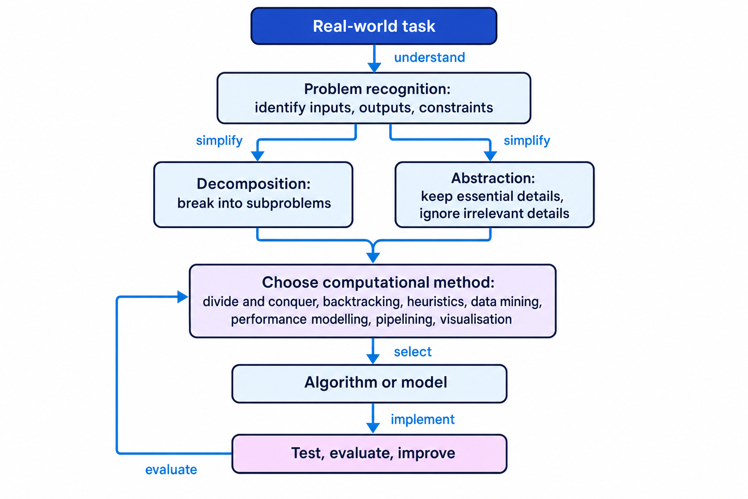
The usual journey is: understand the real-world task, recognise the computational part, simplify it, choose a method, then test and improve the solution.

Features that make a problem computationally solvable

A problem is more suitable for computational methods when:

• Inputs can be represented as data, such as numbers, text, records, images, graph nodes or sensor readings.
• Outputs are clear, such as a route, classification, timetable, prediction or decision.
• Rules and constraints are precise enough for a computer to test.
• The solution can be described as a finite sequence of steps, an algorithm.
• There is repetition, scale or complexity that makes automation useful.
• The time, memory and hardware requirements are feasible.

Some problems are still difficult even if they are computational. For example, finding the absolute best delivery route for many locations may be too slow using a brute-force search, so you may need heuristics or approximation.

Problem recognition

Problem recognition means spotting the underlying computational problem inside a real-world description.

Common problem types include:

• Searching: finding an item, path or valid solution.
• Sorting: putting data into a required order.
• Optimisation: finding the best solution according to a measure, such as shortest time or lowest cost.
• Classification: assigning data to categories, such as spam or not spam.
• Simulation: modelling a system to predict behaviour.
• Pattern discovery: finding useful relationships in data.

A useful structure is IPO: input, process, output.

Problem decomposition

Decomposition means breaking a large problem into smaller subproblems. Each subproblem should be easier to understand, solve, test and maintain.

For example, a school timetable system could be decomposed into:

• store teachers, rooms, subjects and classes
• check room availability
• check teacher availability
• assign lessons to time slots
• detect clashes
• produce printable timetables

Each subproblem can then be designed as a separate module, function or procedure.

Divide and conquer

Divide and conquer is a special form of decomposition. The problem is divided into smaller versions of the same problem, those smaller problems are solved, and the results are combined.

A recursive algorithm is an algorithm that calls itself. Many divide-and-conquer algorithms are recursive. A base case is the smallest case that can be solved directly, stopping the recursion.

Examples include:

• Binary search: repeatedly halve a sorted list.
• Merge sort: split a list, sort both halves, then merge them.
• Some graph and geometry algorithms.

Here is OCR-style pseudocode for recursive binary search on a sorted array:

function binarySearch(items, target, low, high)
    if low > high then
        return -1
    endif

    mid = (low + high) DIV 2

    if items[mid] == target then
        return mid
    elseif items[mid] < target then
        return binarySearch(items, target, mid + 1, high)
    else
        return binarySearch(items, target, low, mid - 1)
    endif
endfunction

Abstraction

Abstraction means removing unnecessary detail so you can focus on the important features of a problem.

A model is a simplified representation of something real. Good abstraction keeps details that affect the answer and ignores details that do not.

Backtracking

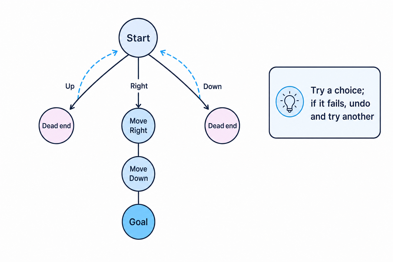
Backtracking is a search technique that builds a solution one choice at a time. If a partial solution cannot lead to a valid full solution, the algorithm undoes that choice and tries another.

It is useful for constraint problems such as mazes, Sudoku, N-Queens, graph colouring and timetable construction.

Data mining

Data mining means using computational techniques to discover patterns, relationships or unusual cases in large data sets.

It may involve:

• classification, such as predicting whether an email is spam
• clustering, such as grouping similar customers
• association, such as finding products often bought together
• anomaly detection, such as spotting suspicious transactions

Heuristics

A heuristic is a rule of thumb that gives a good-enough solution quickly, but does not guarantee the best possible solution.

Heuristics are useful when an exact algorithm would be too slow, especially for large optimisation or search problems.

Performance modelling

Performance modelling means predicting how a system or algorithm will behave before, or while, building it.

Models can use test measurements, equations, simulations or Big-O notation. Big-O describes how runtime or memory grows as input size increases:

• $O(1)$ — constant
• $O(\log n)$ — logarithmic
• $O(n)$ — linear
• $O(n^k)$ — polynomial
• $O(2^n)$ — exponential

Pipelining

Pipelining means splitting a process into stages so that different items can be processed by different stages at the same time.

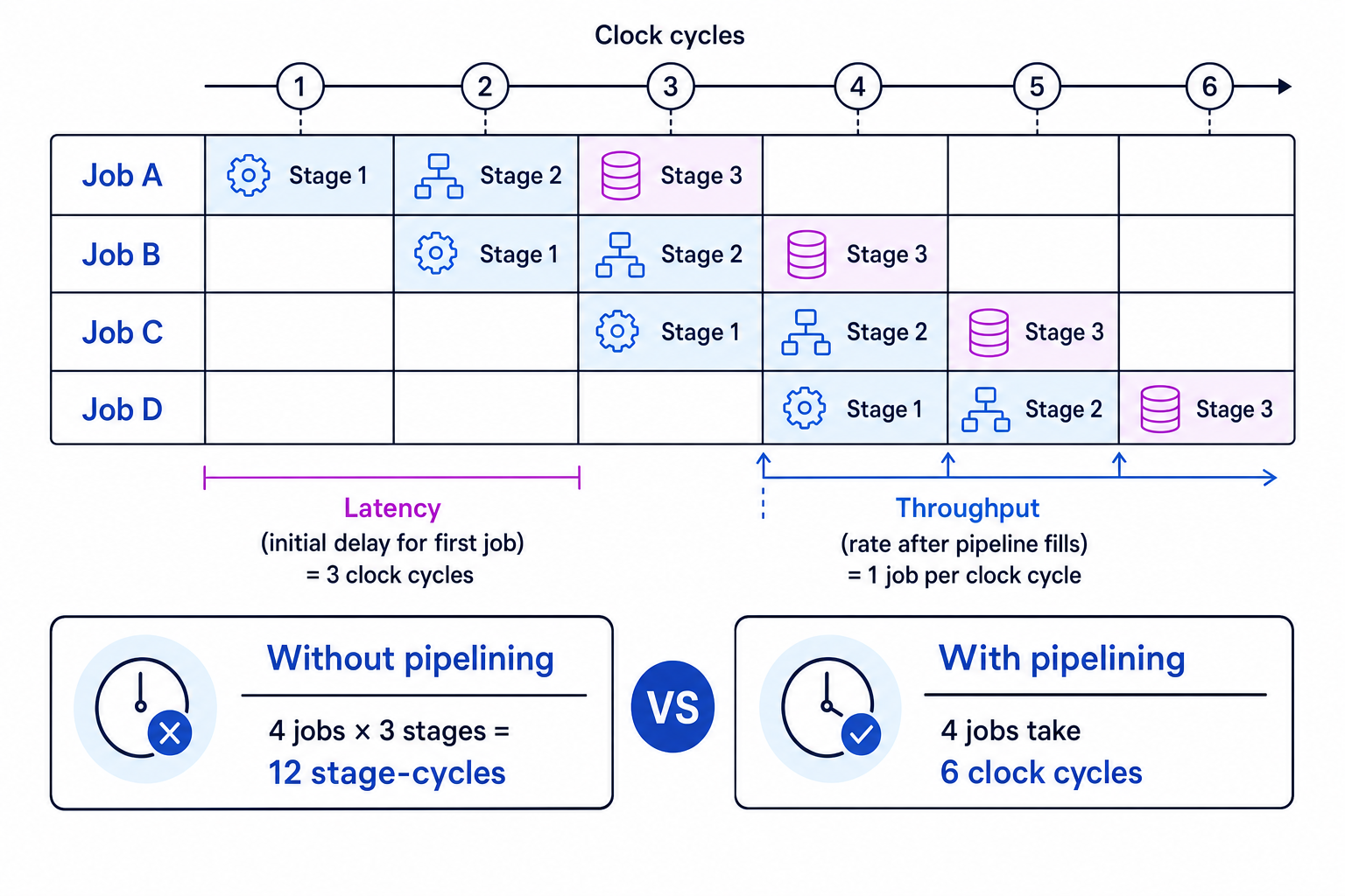
A stage is one part of the process. Latency is the time for one item to pass through the whole pipeline. Throughput is the number of completed items per unit time. A bottleneck is the slowest stage that limits the whole pipeline.

In Component 01 you meet this with processor pipelines, such as overlapping fetch, decode and execute. The same idea applies more widely to data processing and manufacturing.

Visualisation

Visualisation means representing data or structure graphically so patterns are easier to see. Examples include graphs, charts, heat maps, network diagrams, Gantt charts and flowcharts.

Visualisation helps humans make decisions; it does not automatically prove that a solution is correct.